The role of central bank capital revisited - ECB - Monte Carlo Simulations
https://www.econstor.eu/bitstream/10419/152826/1/ecbwp0392.pdf
This paper by Bindseil, Manzanares, and Weller (2004) is from the ECB working paper series which runs a series of Monte Carlo analyses to study the role of central bank capital (amongst other interesting analysis). They focus on the relationship between the Central Bank’s balance sheet structure and inflation performance. They conclude that “Capital thus remains a key tool to ensure that central banks are unconstrained in their focus on price stability in monetary policy decisions.”
One of the key arguments which comes out of this paper is that a central banks net worth is important.
They start by describing a simple balance-sheet based model of a central bank, asusming no liquidity constraints. We describe the model below:
- Assets:
- Monetary policy operations $M$
- Interpret as residual of the balance sheet, and thus will earn a rate of $i_M %$.
- CB is assumed to follow a simplified Taylor rule $i_{M,t} = 4 + 1.5(\pi_{t-1} - 2)$. A floor of zero is assumed.
- Other financial assets $F$
- This includes foreign exchange reserves (gold) and potentially domestic financial assets.
- Assume remunerated at $ i_F % $
- Assume that $i_{F,t} = i_{M,t} + \rho + \omega_t$ where $\omega_t \sim \mathcal{N}(0, \,\sigma_{\omega}^{2}) $ and $\rho$ is some level of asset revaluation gains/losses
- Monetary policy operations $M$
- Liabilities:
- Banknotes $B$
- Function of finlation, and will tend to increase over time
- $ B_t = B_{t-1} + B_{t-1}\frac{(2+\pi_t)}{100} + \epsilon_t $ where $\pi_t$ is the inflation rate, $2$ is the assumed real interest rate and $\epsilon_t \sim \mathcal{N}(0, \,\sigma_{\epsilon}^{2}) $.
- Real interest rate is assumed to be exogenous (outside of model)
- Capital $C$
- Capital is a function of previous years capital and previous year’s profit & loss (P&L)
- Assumed that if previous years profit, $P_{t_1} > 0 $ then there’ll be an $\alpha$ proportion of profit sharing and thus: $C_t = C_{t-1} + \alpha P_{t-1} $ else the full loss is born so $C_t = C_{t-1} + P_{t-1} $
- Banknotes $B$
To model inflation, a Wicksellian relationship is assumed:
\[\pi_{t+1} = \pi_t + \beta (2 + \pi_t - i_{M,t}) + \mu_t\]where $ \mu_t \sim \mathcal{N}(0, \,\sigma_{\mu}^{2}) $, and $\beta$ is a constant parameter.
Taking all of this, we can build the full time-series model:
\(\pi_{t+1} = \pi_t + \beta (2 + \pi_t - i_{M,t}) + \mu_t\) \(q_t = (1+\frac{\pi_t}{100})q_{t-1}\) \(F_t = F\)
\[C_t = \begin{cases} C_{t-1} + \alpha P_{t-1}, \text{if $P_{t-1} > 0$} \\ C_{t-1} + P_{t-1}, \text{if $P_{t-1} < 0$} \end{cases}\] \[B_t = B_{t-1} + B_{t-1} \frac{(2+\pi_t)}{100} + \epsilon_t\] \[i_{M,t} = \begin{cases} \max(4+1.5(\pi_{t-1} -2, 0), \text{if $\max(4+1.5(\pi_{t-1} -2, 0) < \frac{\pi_{t-1}}{\beta} + 2 + \pi_{t-1}$} \\ \frac{\pi_{t-1}}{\beta} + 2 + \pi_{t-1}, \text{if $\max(4+1.5(\pi_{t-1} -2, 0) > \frac{\pi_{t-1}}{\beta} + 2 + \pi_{t-1}$} \end{cases}\]\(i_{F,t} = i_{M,t} + \rho + \omega_t\) \(M_t = B_t + C_t - F_t\) \(P_t = i_{M,t}M_t + i_{F,t}F_t - q_t\)
where $q_t$ is cost of running the central bank, $\alpha, \beta,$ and $\rho$ are parameters.
What it all boils down to, from a Monte Carlo perspective, is the randomness introduced through $\mu_t, \omega_t,$ and $\epsilon_t$. Under a given set of initial conditions for $(M_0, F_0, B_0, C_0, \pi_0, i_0)$ and defined parameters $(\alpha, \beta, \rho, \sigma_{\epsilon}^2, \sigma_{\omega}^2, \sigma_{\mu}^2 )$, we can run $N$ simulations over $t$ periods, and study the distributional outcomes to understand expected average behaviour as well as “unlikely but still possible” scenarios.
In this, I’ll look to implement the base model they present in the paper, and explore a few of the interesting results that they present. In a follow-up note, I’ll look to run some parameter analysis, as this paper worked within a defined set of constant parameters, so it would be an interesting exercise to study the system stability and sensitivity to parameter choices.
import pandas as pd
import numpy as np
import matplotlib.pyplot as plt
import random as random
def pi_f(prev, beta, i_m, sigma_u):
    """
    Produces the current period inflation

    Args:
        prev: Previous period inflation
        beta: Constant parameter
        i_m: Previous period monetary rate
        sigma_u: Inflation variance
    Returns:
        Float

    """

    prev *= 100 # Note that the paper wasn't consistent with scaling
    i_m *= 100
    return (prev + beta*(2 + prev - i_m) + np.random.normal(0, sigma_u)) / 100

def q_t(pi, prev):
    """
    Produces the current period cost of operations

    Args:
        prev: Previous period cost
        pi: Current period inflation

    Returns:
        Float

    """

    pi*= 100

    return ((1+pi/100)*prev)

def c_t(alpha, prev, p_t1):
    """
    Produces the current period capital

    Args:
        alpha: Constant parameter
        prev: Previous period capital
        p_t1: Previous period profit

    Returns:
        Float

    """

    if p_t1 >= 0:
        return prev + alpha*p_t1
    else:
        return prev + p_t1

def i_mt(pi, beta):
    """
    Produces the current period monetary rate

    Args:
        pi: Previous period  inflation
        beta: Constant parameter

    Returns:
        Float
    """

    pi *= 100

    if (max(4 + 1.5*(pi-2), 0) < pi/beta + 2 + pi):
        im = max(4 + 1.5*(pi-2), 0) / 100
    else:
        im = (pi/beta + 2 + pi) / 100

    return max(im, 0)

def i_mt_tilde(pi, beta, theta):
    """
    Produces the current period monetary rate
    under a modified interest rate rule

    Args:
        pi: Previous period  inflation
        beta: Constant parameter

    Returns:
        Float
    """

    pi *= 100

    if (max(4 + 1.5*(pi-2), 0) < pi/beta + 2 + pi):
        im = max(4 + 1.5*(pi-2), 0) / 100
    else:
        im = (pi/beta + 2 + pi) / 100

    return min(im, (0.04+theta))


def i_ft(i_m, rho, sigma_w):
    """
    Produces the current period financial asset rate

    Args:
        i_m: Current period monetary rate
        rho: Constant parameter
        sigma_w: Volatility of rate

    Returns:
        Float
    """

    i_m *= 100

    return (i_m + rho + np.random.normal(0, sigma_w)) / 100

def b_t(prev, pi, sigma_e):
    """
    Produces the current period banknote value

    Args:
        prev: Previous period banknote value
        pi: Current period inflation
        sigma_e: Volatility of rate

    Returns:
        Float
    """

    pi *= 100

    return prev + prev*(2 + pi)/100  + np.random.normal(0, sigma_e)

def m_t(b,c,f):
    """
    Produces the current period monetary value

    Args:
        b: Current period banknote value
        c: Current period capital value
        f: Current period other financial assets values

    Returns:
        Float
    """

    return b + c - f

def p_t(i_m, m, i_f, f, q):
    """
    Produces the current period profit

    Args:
        i_m: Current period monetary rate
        M: Current period monetary value
        i_f: Current period financial rate
        f: Current period other financial values
        q: Current period cost of operations

    Returns:
        Float
    """

    return i_m*m + i_f*f - q

def run_simulation(t, m0, b0, c0, f0, pi0, q0, i0,
                  rho, alpha, beta, theta, sigma_e, sigma_w,
                  sigma_u, use_theta=False, loss_scenario=False):
    """
    Runs one simulation of the central bank balance sheet
    model

    Args:
        t: Number of time periods
        m0: Initial monetary value
        b0: Initial banknotes value
        c0: Initial capital value
        f0: Initial other financial assets value
        pi0: Initial inflation rate
        q0: Initial cost of operation
        i0: Initial interest rate
        rho: Constant parameter
        alpha: Constant parameter
        beta: Constant parameter
        theta: Constant parameter
        sigma_e: Banknotes volatility
        sigma_w: Financial assets volatility
        sigma_u: Inflation volatility
        use_theta: True/False flag for theta model
        loss_scenario: True/False flag for loss profit function


    Returns:
        array of variables of interest
    """

    pi = [np.nan]*t
    q = [np.nan]*t
    f = [np.nan]*t
    c = [np.nan]*t
    b = [np.nan]*t
    i_m = [np.nan]*t
    i_f = [np.nan]*t
    m = [np.nan]*t
    p = [np.nan]*t

    m[0] = m0
    b[0] = b0
    f[0] = f0
    pi[0] = pi0
    i_m[0] = i0
    i_f[0] = i0
    q[0] = q0
    c[0] = c0
    p[0] = p_t(i0, m0, i0, f0, q0)

    loss_maker = False
    for i in np.arange(t):

        if i == 0:
            pass
        else:
            pi[i] = pi_f(pi[i-1], beta, i_m[i-1], sigma_u)
            q[i] = q_t(pi[i], q[i-1])
            f[i] = f[i-1]
            b[i] = b_t(b[i-1], pi[i], sigma_e)
            c[i] = c_t(alpha, c[i-1], p[i-1])

            if use_theta:
                if c[i] < 0 or loss_maker is True:
                    i_m[i] = min(i_mt(pi[i-1], beta), 0.04+theta)
                else:
                    i_m[i] = i_mt(pi[i-1], beta)
            else:
                i_m[i] = i_mt(pi[i-1], beta)

            i_f[i] = i_ft(i_m[i], rho, sigma_w)
            m[i] = m_t(b[i],c[i],f[i])
            p[i] = p_t(i_m[i], m[i], i_f[i], f[i], q[i])

            if loss_scenario:
                loss_maker =  random.random() < 0.1
                if loss_maker:
                    p[i] = -0.33 * b[i]

    return pi, q, f, b, c, i_m, i_f, m, p
Scenario 1
In scenario 1, we have a profit making central bank which has positive capital.
# Initial settings
m0 = 120 # note that m0 = b0+c0
b0 = 100
c0 = 20
f0 = 0
pi0 = 0.02
q0 = 1
i0 = 0.04

# Constant parameters
rho = 0.02
sigma_e = 1
sigma_w = 0.5
sigma_u = 0.5
alpha = 0.5
beta = 0.2
theta = -0.01

pi_full = []
q_full = []
f_full = []
b_full = []
c_full = []
im_full = []
if_full = []
m_full = []
p_full  = []

for j in np.arange(10000):
    a,b,c,d,e,f,g,h,i = run_simulation(100,  m0, b0, c0, f0, pi0, q0, i0,
                  rho, alpha, beta, theta, sigma_e, sigma_w,
                  sigma_u, use_theta=False)

    pi_full.append(a)
    q_full.append(b)
    f_full.append(c)
    b_full.append(d)
    c_full.append(e)
    im_full.append(f)
    if_full.append(g)
    m_full.append(h)
    p_full.append(i)
plt.figure(figsize=(15,10))
pd.DataFrame(pi_full).T.quantile(0.95, axis=1).plot(label='Inflation 95%', color='r', linestyle='-.')
pd.DataFrame(pi_full).T.quantile(0.05, axis=1).plot(label='Inflation 5%', color='r', linestyle='--')
pd.DataFrame(pi_full).T.quantile(0.5, axis=1).plot(label='Inflation Median', color='r', linewidth=6)

pd.DataFrame(im_full).T.quantile(0.95, axis=1).plot(label='Interest 95%', color='k', linestyle='-.')
pd.DataFrame(im_full).T.quantile(0.05, axis=1).plot(label='Interest 5%', color='k', linestyle='--')
pd.DataFrame(im_full).T.quantile(0.5, axis=1).plot(label='Interest Median', color='k', linewidth=6)
plt.ylim(-0.02, 0.11)

plt.ylabel('Simulation Period', fontsize=12)
plt.xlabel('Annualised Rate', fontsize=12)
plt.title('Time-series of inflation and interest rates', fontsize=16)
plt.legend()
plt.tight_layout()
plt.show()
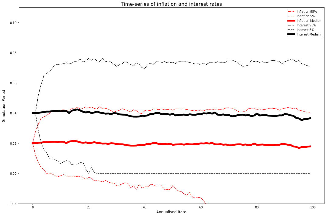
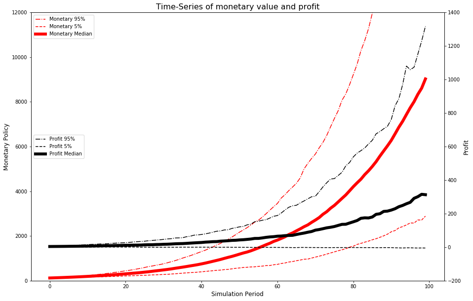
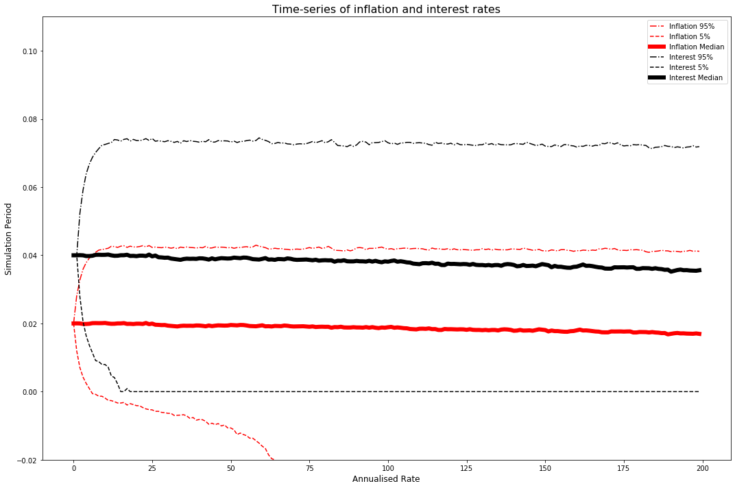
The primary take away from these charts is that, under this model, even a central bank which is currently profitable, with positive capital, there is a non-zero probability that the central bank gets stuck in a deflationary situation permanently. This drives income and profit to zero. The model has assumed that there is a fixed level targeting of inflation, that is also used in setting the yield on monetary policy operations. Under an actual central bank, they have the option of changing their behaviour or “policy”, and thus could respond to a deflationary scenario by perhaps targeting higher inflation rates.
fig, ax = plt.subplots(figsize=(15,10))

ax2 = ax.twinx()

pd.DataFrame(m_full).T.quantile(0.95, axis=1).plot(ax=ax, label='Monetary 95%', color='r', linestyle='-.')
pd.DataFrame(m_full).T.quantile(0.05, axis=1).plot(ax=ax, label='Monetary 5%', color='r', linestyle='--')
pd.DataFrame(m_full).T.quantile(0.5, axis=1).plot(ax=ax, label='Monetary Median', color='r', linewidth=6)

pd.DataFrame(p_full).T.quantile(0.95, axis=1).plot(ax=ax2, label='Profit 95%', color='k', linestyle='-.')
pd.DataFrame(p_full).T.quantile(0.05, axis=1).plot(ax=ax2, label='Profit 5%', color='k', linestyle='--')
pd.DataFrame(p_full).T.quantile(0.5, axis=1).plot(ax=ax2, label='Profit Median', color='k', linewidth=6)


ax.set_ylabel('Monetary Policy', fontsize=12)
ax2.set_ylabel('Profit', fontsize=12)
ax.set_xlabel('Simulation Period', fontsize=12)

ax.set_ylim([0, 12000])
ax2.set_ylim([-200, 1400])
ax.legend(loc='upper left')
ax2.legend(loc='center left')
plt.title('Time-Series of monetary value and profit', fontsize=16)
plt.show()
Scenario 2
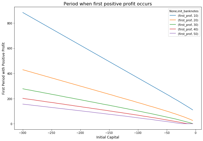
A non-profitable central bank with negative initial capital.
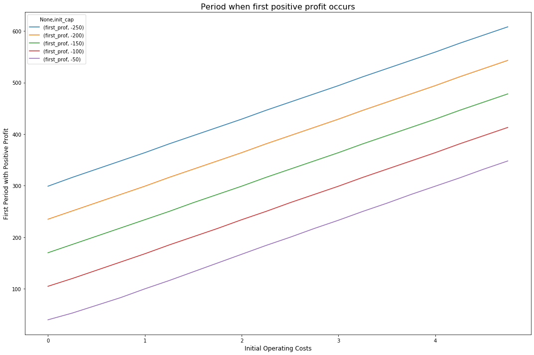
We start with the deterministic scenario, i.e. no random variables. This scenario shows that, under the deterministic scenario, there is always a period in the future in which the central bank generates a profit. This is a function of the models assumed for growth of the banknotes and operating costs. Operating costs grow at only the inflation rate, $\pi_t$ whilst the banknotes grow at the nominal interest rate. Thus, under the given set of assumptions, in the deterministic case, for any given initial values of capital, $C_0$, and operating costs $q_0$, the central bank will eventually turn a positive profit.
m0 = -60
b0 = 20
c0 = -80
f0 = 0
pi0 = 0.02
q0 = 1
i0 = 0.04

# level parameters
rho = 0.02
sigma_e = 0
sigma_w = 0
sigma_u = 0
alpha = 0.5
beta = 0.2
theta = -0.01

init_period = []

# loop over initial banknote value
for bn in [10, 20, 30, 40, 50]:

    # loop over initial capital value
    for cap in np.arange(-300, 0, 5):

        # Note m0 = initial banknote + initial capital
        a,b,c,d,e,f,g,h,i = run_simulation(1000, cap+bn, bn, cap, f0, pi0, q0, i0,
                      rho, alpha, beta, theta, sigma_e, sigma_w,
                      sigma_u, use_theta=False)

        init_profit = next(x[0] for x in enumerate(i) if x[1] > 0)

        init_period.append((bn, cap, init_profit))
pos_prof = pd.DataFrame(init_period)
pos_prof.columns = ['init_banknotes', 'init_cap', 'first_prof']
pos_prof.pivot(index='init_cap', columns='init_banknotes').plot(figsize=(10,7))
plt.ylabel('First Period with Positive Profit', fontsize=12)
plt.xlabel('Initial Capital', fontsize=12)
plt.title('Period when first positive profit occurs', fontsize=16)
plt.tight_layout()
plt.show()
init_period = []

# loop over initial operating costs
for qn in np.arange(0, 5, 0.25):

    # loop over initial capital values
    for cap in [-250, -200, -150, -100, -50]:

        a,b,c,d,e,f,g,h,i = run_simulation(1000,  b0+cap, b0, cap, f0, pi0, qn, i0,
                      rho, alpha, beta, theta, sigma_e, sigma_w,
                      sigma_u, use_theta=False)

        init_profit = next(x[0] for x in enumerate(i) if x[1] > 0)

        init_period.append((qn, cap, init_profit))
pos_prof = pd.DataFrame(init_period)
pos_prof.columns = ['init_opcosts', 'init_cap', 'first_prof']
pos_prof.pivot(index='init_opcosts', columns='init_cap').plot(figsize=(15,10))
plt.ylabel('First Period with Positive Profit', fontsize=12)
plt.xlabel('Initial Operating Costs', fontsize=12)
plt.title('Period when first positive profit occurs', fontsize=16)
plt.tight_layout()
plt.show()
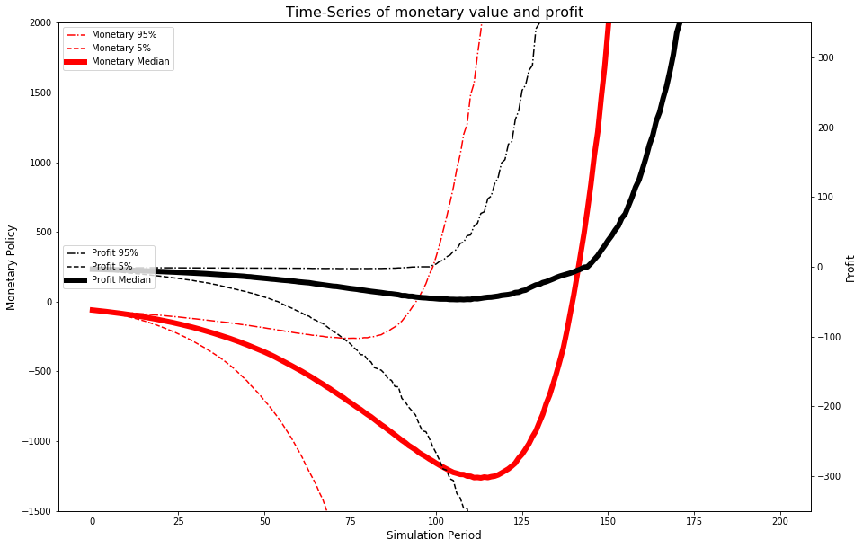
Now we add back in the random variables, and return to Monte Carlo analysis. We find that, in the median case, a negative central bank, with given variable shocks, will turn a profit at approximately period 140 in the simulation.
m0 = -60
b0 = 20
c0 = -80
f0 = 0
pi0 = 0.02
q0 = 1
i0 = 0.04

# level parameters
rho = 0.02
sigma_e = 1
sigma_w = 0.5
sigma_u = 0.5
alpha = 0.5
beta = 0.2
theta = -0.01

pi_full = []
q_full = []
f_full = []
b_full = []
c_full = []
im_full = []
if_full = []
m_full = []
p_full  = []

for j in np.arange(10000):
    a,b,c,d,e,f,g,h,i = run_simulation(200, m0, b0, c0, f0, pi0, q0, i0,
                  rho, alpha, beta, theta, sigma_e, sigma_w,
                  sigma_u, use_theta=False)

    pi_full.append(a)
    q_full.append(b)
    f_full.append(c)
    b_full.append(d)
    c_full.append(e)
    im_full.append(f)
    if_full.append(g)
    m_full.append(h)
    p_full.append(i)
plt.figure(figsize=(15,10))
pd.DataFrame(pi_full).T.quantile(0.95, axis=1).plot(label='Inflation 95%', color='r', linestyle='-.')
pd.DataFrame(pi_full).T.quantile(0.05, axis=1).plot(label='Inflation 5%', color='r', linestyle='--')
pd.DataFrame(pi_full).T.quantile(0.5, axis=1).plot(label='Inflation Median', color='r', linewidth=6)

pd.DataFrame(im_full).T.quantile(0.95, axis=1).plot(label='Interest 95%', color='k', linestyle='-.')
pd.DataFrame(im_full).T.quantile(0.05, axis=1).plot(label='Interest 5%', color='k', linestyle='--')
pd.DataFrame(im_full).T.quantile(0.5, axis=1).plot(label='Interest Median', color='k', linewidth=6)
plt.ylim(-0.02, 0.11)

plt.ylabel('Simulation Period', fontsize=12)
plt.xlabel('Annualised Rate', fontsize=12)
plt.title('Time-series of inflation and interest rates', fontsize=16)
plt.legend()
plt.tight_layout()
plt.show()
fig, ax = plt.subplots(figsize=(15,10))

ax2 = ax.twinx()

pd.DataFrame(m_full).T.quantile(0.95, axis=1).plot(ax=ax, label='Monetary 95%', color='r', linestyle='-.')
pd.DataFrame(m_full).T.quantile(0.05, axis=1).plot(ax=ax, label='Monetary 5%', color='r', linestyle='--')
pd.DataFrame(m_full).T.quantile(0.5, axis=1).plot(ax=ax, label='Monetary Median', color='r', linewidth=6)

pd.DataFrame(p_full).T.quantile(0.95, axis=1).plot(ax=ax2, label='Profit 95%', color='k', linestyle='-.')
pd.DataFrame(p_full).T.quantile(0.05, axis=1).plot(ax=ax2, label='Profit 5%', color='k', linestyle='--')
pd.DataFrame(p_full).T.quantile(0.5, axis=1).plot(ax=ax2, label='Profit Median', color='k', linewidth=6)


ax.set_ylabel('Monetary Policy', fontsize=12)
ax2.set_ylabel('Profit', fontsize=12)
ax.set_xlabel('Simulation Period', fontsize=12)

ax.set_ylim([-1500, 2000])
ax2.set_ylim([-350, 350])
ax.legend(loc='upper left')
ax2.legend(loc='center left')
plt.title('Time-Series of monetary value and profit', fontsize=16)
plt.show()
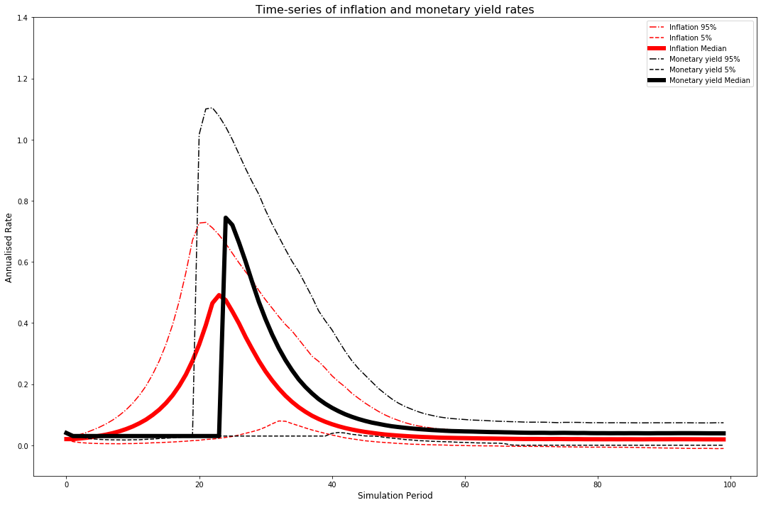
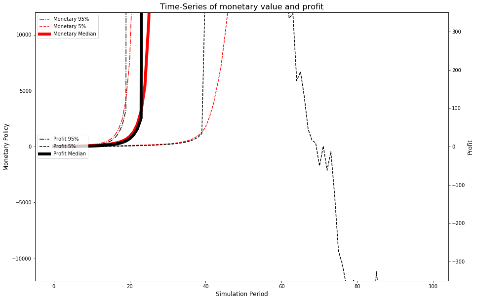
Modified interest rate policy
Now we look at the scenario where, when a central bank has negative capital, we substitute the Taylor rule interest rate with:
\[\tilde{i}_{M,t} = \min(4+\theta, i_{M,t})\]Note, I haven’t been able to exactly replicate the results based on the description given in the paper. There’s likely a small detail in the treatment which has been left out of the description which is giving slightly different results.
In this scenario, the central bank swings back to positive profitability much faster, in “exchange” for higher inflation rates. This occurs in around period 40 of the simulation.
m0 = 20
b0 = 100
c0 = -80
f0 = 0
pi0 = 0.02
q0 = 1
i0 = 0.04

# level parameters
rho = 0.02
sigma_e = 1
sigma_w = 0.5
sigma_u = 0.5
alpha = 0.5
beta = 0.2
theta = -0.01

pi_full = []
q_full = []
f_full = []
b_full = []
c_full = []
im_full = []
if_full = []
m_full = []
p_full  = []

for j in np.arange(10000):
    a,b,c,d,e,f,g,h,i = run_simulation(100,  m0, b0, c0, f0, pi0, q0, i0,
                  rho, alpha, beta, theta, sigma_e, sigma_w,
                  sigma_u, use_theta=True)

    pi_full.append(a)
    q_full.append(b)
    f_full.append(c)
    b_full.append(d)
    c_full.append(e)
    im_full.append(f)
    if_full.append(g)
    m_full.append(h)
    p_full.append(i)
plt.figure(figsize=(15,10))
pd.DataFrame(pi_full).T.quantile(0.95, axis=1).plot(label='Inflation 95%', color='r', linestyle='-.')
pd.DataFrame(pi_full).T.quantile(0.05, axis=1).plot(label='Inflation 5%', color='r', linestyle='--')
pd.DataFrame(pi_full).T.quantile(0.5, axis=1).plot(label='Inflation Median', color='r', linewidth=6)

pd.DataFrame(im_full).T.quantile(0.95, axis=1).plot(label='Monetary yield 95%', color='k', linestyle='-.')
pd.DataFrame(im_full).T.quantile(0.05, axis=1).plot(label='Monetary yield 5%', color='k', linestyle='--')
pd.DataFrame(im_full).T.quantile(0.5, axis=1).plot(label='Monetary yield Median', color='k', linewidth=6)
plt.ylim(-0.1, 1.40)

plt.xlabel('Simulation Period', fontsize=12)
plt.ylabel('Annualised Rate', fontsize=12)
plt.title('Time-series of inflation and monetary yield rates', fontsize=16)
plt.legend()
plt.tight_layout()
plt.show()
fig, ax = plt.subplots(figsize=(15,10))

ax2 = ax.twinx()

pd.DataFrame(m_full).T.quantile(0.95, axis=1).plot(ax=ax, label='Monetary 95%', color='r', linestyle='-.')
pd.DataFrame(m_full).T.quantile(0.05, axis=1).plot(ax=ax, label='Monetary 5%', color='r', linestyle='--')
pd.DataFrame(m_full).T.quantile(0.5, axis=1).plot(ax=ax, label='Monetary Median', color='r', linewidth=6)

pd.DataFrame(p_full).T.quantile(0.95, axis=1).plot(ax=ax2, label='Profit 95%', color='k', linestyle='-.')
pd.DataFrame(p_full).T.quantile(0.05, axis=1).plot(ax=ax2, label='Profit 5%', color='k', linestyle='--')
pd.DataFrame(p_full).T.quantile(0.5, axis=1).plot(ax=ax2, label='Profit Median', color='k', linewidth=6)


ax.set_ylabel('Monetary Policy', fontsize=12)
ax2.set_ylabel('Profit', fontsize=12)
ax.set_xlabel('Simulation Period', fontsize=12)

ax.set_ylim([-12000, 12000])
ax2.set_ylim([-350, 350])
ax.legend(loc='upper left')
ax2.legend(loc='center left')
plt.title('Time-Series of monetary value and profit', fontsize=16)
plt.show()
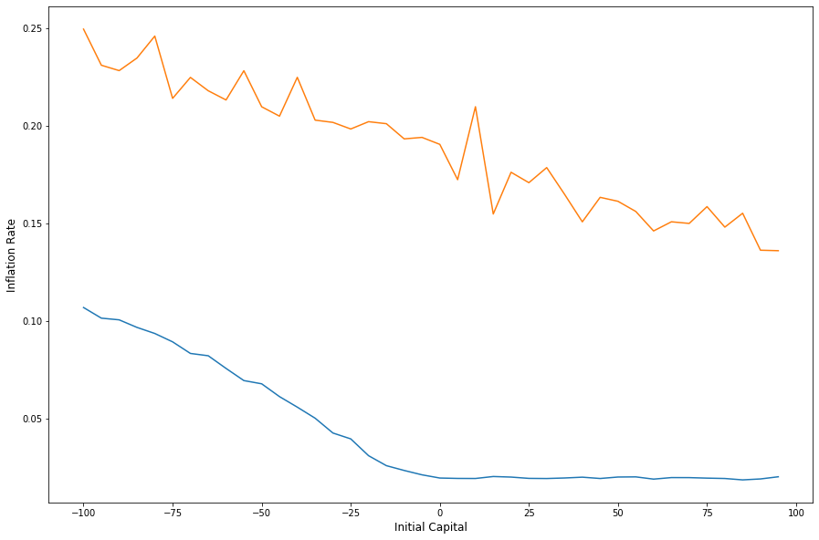
In this setting, the paper introduced a “loss-making” episode. In each period, there is a 10% probability that the central bank makes an annual loss of 33% of the banknote values.
b0 = 100
f0 = 0
pi0 = 0.02
q0 = 1
i0 = 0.04

# level parameters
rho = 0.02
sigma_e = 1
sigma_w = 0.5
sigma_u = 0.5
alpha = 0.5
beta = 0.2
theta = -0.01

avg_inflation = []
avg_inflation_loss = []

for cap in np.arange(-100, 100, 5):
    cap_infl = []
    cap_infl_loss = []
    m0 = b0 + cap
    for j in np.arange(200):
        a,b,c,d,e,f,g,h,i = run_simulation(100, m0, b0, cap, f0, pi0, q0, i0,
                      rho, alpha, beta, theta, sigma_e, sigma_w,
                      sigma_u, use_theta=True)

        cap_infl.append(np.mean(a))

        a,b,c,d,e,f,g,h,i = run_simulation(100, m0, b0, cap, f0, pi0, q0, i0,
                      rho, alpha, beta, theta, sigma_e, sigma_w,
                      sigma_u, use_theta=True, loss_scenario=True)

        cap_infl_loss.append(np.mean(a))

    avg_inflation.append(np.median(cap_infl))
    avg_inflation_loss.append(np.median(cap_infl_loss))


avg_inflation_base = pd.DataFrame([np.arange(-100,100,5), avg_inflation]).T
avg_inflation_base.columns=['init_cap', 'avg_infl']
avg_inflation_base.set_index(['init_cap'], inplace=True)

avg_inflation_loss = pd.DataFrame([np.arange(-100,100,5), avg_inflation_loss]).T
avg_inflation_loss.columns=['init_cap', 'avg_infl_loss']
avg_inflation_loss.set_index(['init_cap'], inplace=True)
plt.figure(figsize=(15,10))
plt.plot(avg_inflation_base, label='Median of Average Inflation')
plt.plot(avg_inflation_loss, label='Median of Average Inflation (with loss scenario)')
plt.ylabel('Inflation Rate', fontsize=12)
plt.xlabel('Initial Capital', fontsize=12)
Text(0.5, 0, 'Initial Capital')