Cryptocurrency - Empirical Asset Pricing
Cryptocurrency is all the rage again. Bitcoin has been on a strong, steady surge over 2020. In addition, there is an emerging literature which is applying standard empirical asset pricing techniques to cryptocurrency datasets. What better way to jump on the bandwagon, then combine all of them and setup an infrastructure for crypto asset pricing (from an academic viewpoint).
Disclaimer: this is purely my opinion and for research interests/illustrative purposes. It is in no way investment advice, and may not reflect the views of my employer.
Data Cleaning and Calculations
We use coinmetrics.io data (https://coinmetrics.io/community-network-data/), this isn’t a full dataset but the analysis is equally valid on a larger set of data.
In asset pricing literature, there is a “zoo” of anomalies which are used to explain the cross-section of stock returns. We can lean on this for a first pass. Naturally, this is assuming that the same theories and logic from financial markets also apply to cryptocurrency markets. This assumption is not too far of a stretch, as ultimately humans are behind most of the decisions and choices being made in crypto markets and thus any behavioural anomalies that manifest in other markets, we could reasonably expect that they may also manifest in crypto markets.
Additionally, there might be crypto specific risk factors/anomalies which could be researched/considered. The primary issue with studying cross-sectional returns for crypto is only having 6 years of data to study. This makes it very difficult to draw meaningful conclusions about statistical validity / existence of any anomalies/risk factors. Rather, this research can simply provide indications of potential factors/behaviours in crypto markets.
Factors
We broadly categorise our factors into sentiment/momentum, volume and volatility. The factors below all have substantial literatures/seminal papers behind them if interested.
In addition to these base factors, we also construct a “crypto market return”. We construct a daily and monthly measure of the crypto market return using both a value-weighted (market cap) and equal-weighted approach. We use data from Kenneth French’s data library (https://mba.tuck.dartmouth.edu/pages/faculty/ken.french/data_library.html) to get risk free rates.
We filter our data from 2014/01/01 to 2020/12/22. We only take coins with a market cap > $1m.
Sentiment/momentum factors
- Market capitalisation on rebalance date
- Closing Price on rebalance date
- Maximum return over previous month
- Minimum return over previous month
- 1month/3month/6month price momentum
Volume
- 3 Month average daily value
- Amihud’s Illiquidity
Volatility
- Price volality
- Idiosyncratic vol
- Kurtosis
- Price lottery
- Beta measures: equity/gold/crypto market
- Idiosyncratic skewness/expected skewness/total skewness
Papers
https://www.sciencedirect.com/science/article/abs/pii/S026499931931020X
https://papers.ssrn.com/sol3/papers.cfm?abstract_id=3394671
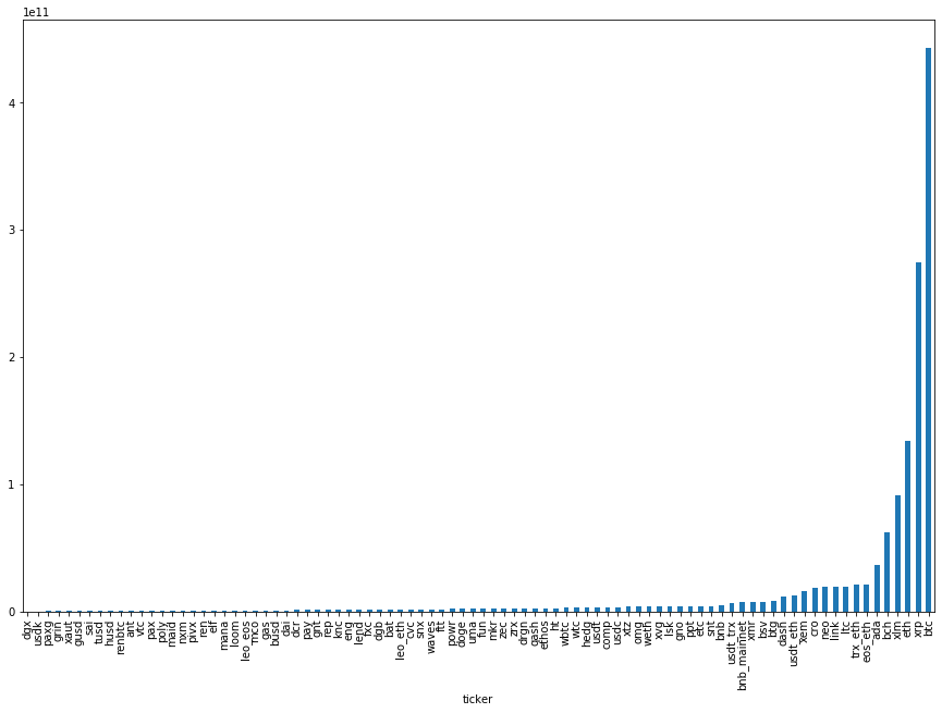
Dataset breadth
We only have a small fraction of the available coin data. This is primarily because we’re using the freely available coinmetrics.io dataset. This will naturally have some biases when looking at cross-sectional return predictability and the existence of asset pricing afctors. Survivorship bias is likely the biggest bias, as well as size bias as you might expect that only the larger/more succesful coins are having their data captured with a sufficient history.
This is a challenging problem in any empirical asset pricing study. For US equities, the CRSP dataset is the standard used in academic literature, as it has been carefully curated and studied for decades. For other equity/asset markets, globally, there is no such universally accepted dataset. This tends to mean that the academic literature has focused on studying US equities. In recent years, Refinitiv/Thomson Reuters and other vendors have increased access to global equity price and market data, but it requires substantially more cleaning and munging to get into an acceptable format.
Risk vs. return of assets/coins
The first question to ask when looking at any asset tends to be, what have historical returns looked like? The second question, if the returns are high, tends to be, and how “risky” is this asset? The commonly accepted measure of risk is price volatility, which is simply the standard deviation of returns over some time period. This is a fairly naive measure of risk, but is easy to calculate so is a good first approximation. More complicated measures such as semi-variance, value-at-risk (VaR) can also be calculated. You don’t want to use one measure of risk, so it’s good practice to put together various risk measures and study each of them. Depending on your use case/application, there will be more suitable definitions of risk that you may want to use. For example, high-frequency traders vs long term investors will likely have very different views of what constitutes an acceptable risk to take in the context of the assets they wish to hold.
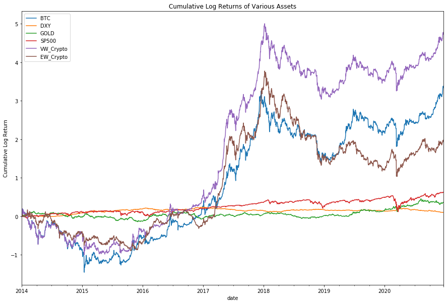
Our first observation is that since 2014, the cumulative returns of cryptocurrencies have absolutely trounced equity markets. On a log scale, returns to cryptocurrencies make equity markets (proxied by S&P500) look almost no risk/bond-like in their behaviour.
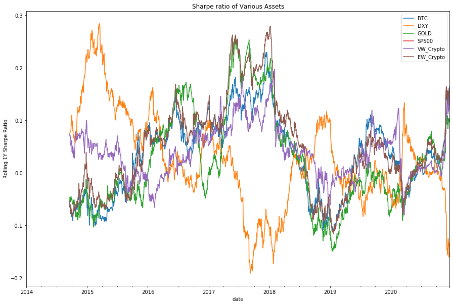
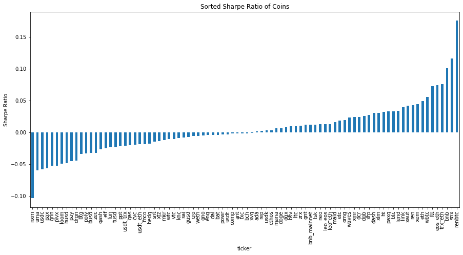
To further expand our study of the nature of these assets, we can look at the Sharpe Ratio, which is effectively a measure of risk-adjusted return. We work in absolute return space (i.e. not relative to a benchmark).
What you’ll notice is that on this scale, the behaviour of cryptocurrency doesn’t look so outstanding anymore. On a risk-adjusted basis, cryptocurrency looks to be generating behaviour similar to standard asset classes such as gold, equities and currency.
Perhaps a more interesting observation is how similar the sharpe ratios between crypto, equities and gold has gotten in 2020. This is potentially a feature of the market downturn in March 2020, and the various changes in market behaviour that have occured due to COVID.
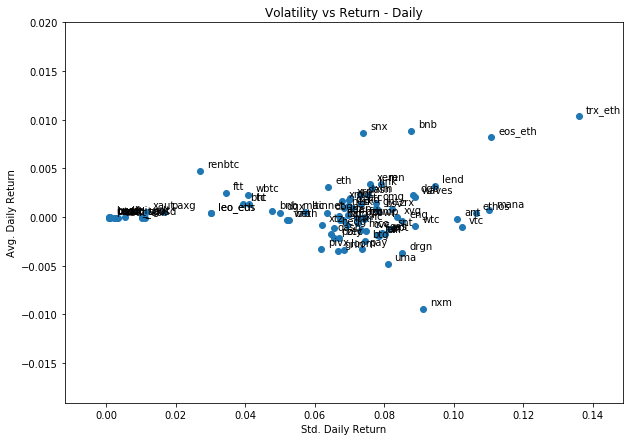
Another way to view risk and return is to plot them against each other. This arises from standard portfolio theory/efficient frontiers and the like.
What you expect/tend to see with assets is that higher risk corresponds to higher returns. We can see that this does tend to occur, and you could almost draw the efficient frontier around the coins.
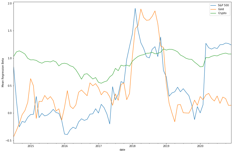
Estimates of beta against SP500, Gold & Crypto value-weighted
Another way to study the relationship between asset classes is to regress the returns against each other. This is commonly known as the CAPM regression beta, but it is simply a standard linear model where our independent variable is the return on asset A and our dependent variable is the return on asset B:
\[r_a = \alpha + \beta_i r_b + \epsilon\]What we do is for each coin, we calculate a running beta at the end of each month using the previous 260 daily return values (with a minimum of 200 observations). We can use benchmarks for equities/gold/crypto to calculate the beta of each coin to each benchmark.
We then can simply take the median value at the end of each month and plot this through time. This will give us an indication on the typical beta in the sample.
What we find is not unsurprising. The median beta to our crypto market returns is positive and between 0.6 and 1.2. We see substantially larger and more volatile values in our S&P500/gold betas. More intruiging is the sharp shift in S&P500 beta to around 1-1.2 where it has stayed for almost all of 2020.
Predicting coin returns
We calculate a series of factors, which we can use to try and predict one-month forward stock returns. In a full study, you would look at multiple frequencies but this is mostly illustrative here.
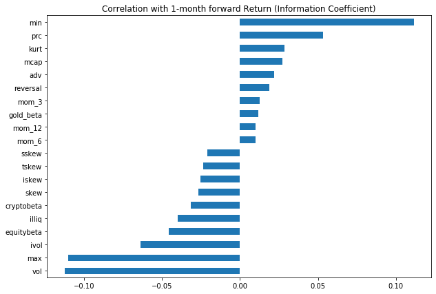
The first common measure is the information coefficient, or the correlation between the factor scores and the one-month forward returns. This gives us an indication for which factors might be useful in predicting future stock returns. However, from an implementation perspective, there’s many, many considerations… transaction costs, turnover, short constraints, to name a few.
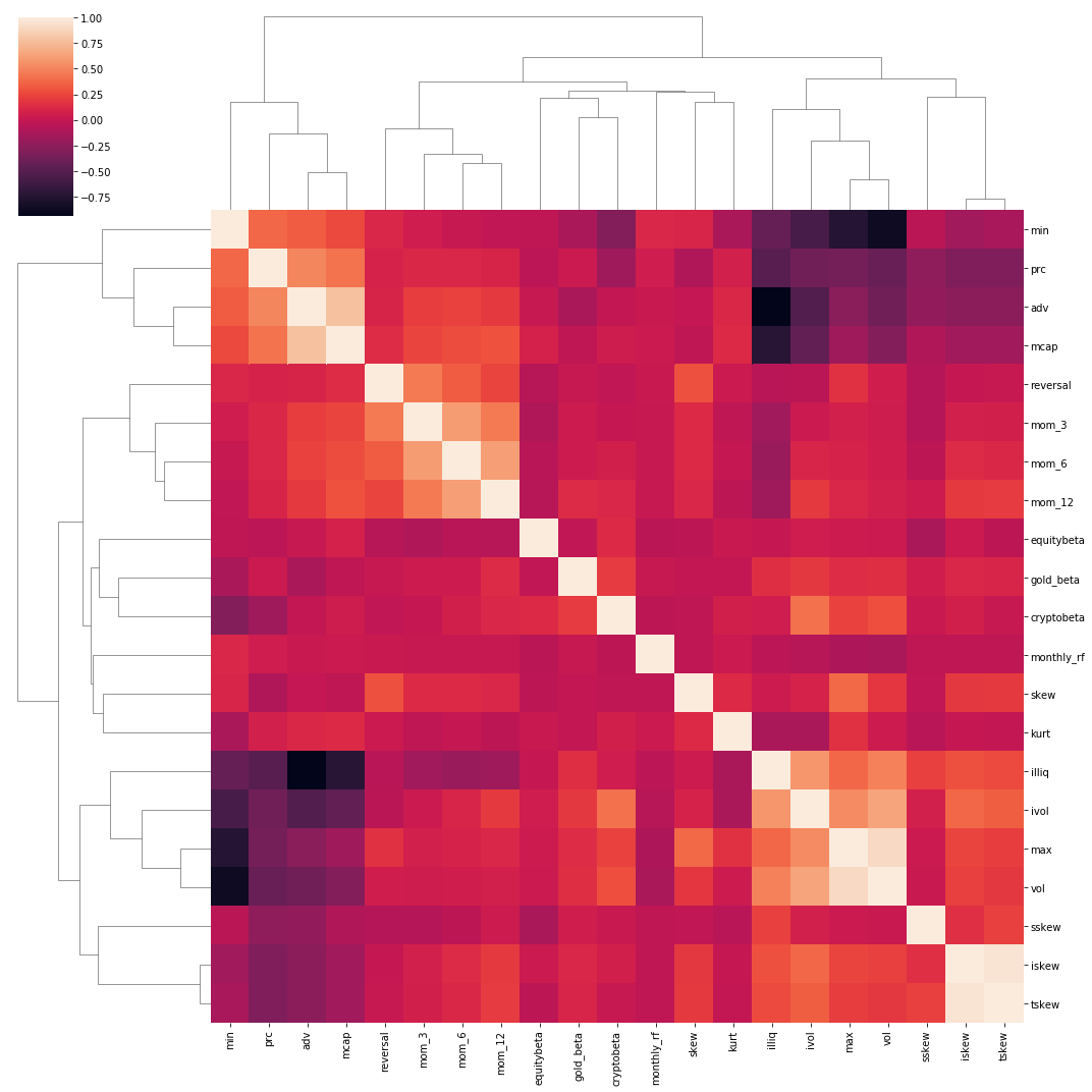
We can also look at the relationship amongst our factors. We can use a dendrogram + heatmap to see if there’s any clustered groups of factors. We see fairly expected results with clustering of momentum factors, beta factors, and then our short-term trading factors.
A common tool in litearature is to look at summary statistics of your factors/variables. This gives you a sense of the scale, and also potentially highlights any outlier/distribution issues you may have to deal with.
| illiq | skew | kurt | max | min | vol | adv | prc | mcap | equitybeta | ivol | iskew | sskew | tskew | gold_beta | cryptobeta | mom_3 | mom_6 | mom_12 | reversal | |
|---|---|---|---|---|---|---|---|---|---|---|---|---|---|---|---|---|---|---|---|---|
| mean | 312.8514 | 0.1151 | 2.1881 | 0.1360 | -0.1214 | 0.0551 | 59,324,704.7266 | 0.7705 | 18.7713 | 0.4090 | 1.0698 | 0.5461 | 12.3359 | 0.3822 | 0.4906 | 0.8962 | 0.0683 | 0.1390 | 0.2855 | 0.0207 |
| std | 1,158.4035 | 0.8707 | 2.6050 | 0.1192 | 0.0873 | 0.0422 | 210,404,538.6605 | 4.2158 | 2.2695 | 0.6393 | 0.3811 | 0.8823 | 38.8270 | 0.9458 | 0.6036 | 0.2625 | 0.5079 | 0.7011 | 1.0042 | 0.2920 |
| skew | 3.5171 | 0.3409 | 1.8674 | 1.3973 | -0.7271 | 0.8190 | 4.5114 | -0.0207 | 0.6741 | 0.1521 | -0.5107 | 0.5395 | 0.5864 | 0.5075 | 0.4373 | -0.9455 | 0.3478 | 0.2244 | 0.0803 | 0.6012 |
| kurt | 16.5495 | 1.6944 | 5.7661 | 3.4935 | 2.4405 | 2.4176 | 25.2469 | -0.5362 | 0.3606 | 0.8562 | 1.1539 | 1.4082 | 2.3305 | 0.6322 | 0.7250 | 2.7936 | 2.3221 | 1.8711 | 1.4487 | 3.5935 |
| count | 36.0000 | 44.0602 | 44.0241 | 44.1566 | 44.1566 | 44.1205 | 36.0843 | 44.2169 | 37.3012 | 30.2289 | 30.2289 | 30.2289 | 30.2289 | 30.2289 | 30.2289 | 30.2289 | 41.8795 | 38.4337 | 31.9277 | 44.2169 |
| min | 0.0001 | -1.7141 | -0.6751 | 0.0016 | -0.3634 | 0.0017 | 170,857.4105 | -7.1226 | 15.1803 | -0.8190 | 0.2622 | -1.0097 | -61.0548 | -1.1095 | -0.5689 | 0.2401 | -0.9632 | -1.3270 | -1.7192 | -0.5641 |
| max | 5,086.6411 | 2.2996 | 11.0954 | 0.5119 | 0.0020 | 0.1781 | 1,308,240,639.7914 | 8.2548 | 24.1141 | 1.7036 | 1.7761 | 2.6050 | 100.6769 | 2.4813 | 1.8168 | 1.2935 | 1.3427 | 1.8044 | 2.5441 | 0.8457 |
| median | 0.1084 | 0.0545 | 1.5419 | 0.1119 | -0.1172 | 0.0506 | 2,253,162.0171 | 0.7036 | 18.3326 | 0.4150 | 1.0869 | 0.4640 | 8.6625 | 0.2920 | 0.4367 | 0.9320 | 0.0485 | 0.1384 | 0.3107 | 0.0018 |
| quantile0.05 | 0.0012 | -1.0884 | -0.2828 | 0.0071 | -0.2458 | 0.0031 | 282,974.3722 | -5.6922 | 15.9418 | -0.4724 | 0.4579 | -0.5034 | -38.4297 | -0.7979 | -0.2634 | 0.4381 | -0.5761 | -0.8020 | -1.0894 | -0.3292 |
| quantile0.25 | 0.0155 | -0.3721 | 0.5694 | 0.0591 | -0.1592 | 0.0303 | 825,318.9527 | -2.1898 | 17.3030 | 0.0573 | 0.8882 | -0.0055 | -5.7353 | -0.2375 | 0.1094 | 0.8273 | -0.2121 | -0.2545 | -0.3392 | -0.1334 |
| quantile0.75 | 1.2623 | 0.5732 | 2.9655 | 0.1763 | -0.0671 | 0.0708 | 13,218,682.3488 | 3.8612 | 20.0003 | 0.7506 | 1.2778 | 0.9592 | 26.3862 | 0.8757 | 0.7996 | 1.0357 | 0.2919 | 0.4756 | 0.8697 | 0.1390 |
| quantile0.95 | 1,521.1662 | 1.4567 | 6.6843 | 0.3297 | -0.0062 | 0.1184 | 269,932,881.8052 | 7.0933 | 22.4340 | 1.2600 | 1.5466 | 1.8803 | 67.5178 | 1.8483 | 1.3720 | 1.2010 | 0.8373 | 1.2024 | 1.7257 | 0.4500 |
Univariate factor trends
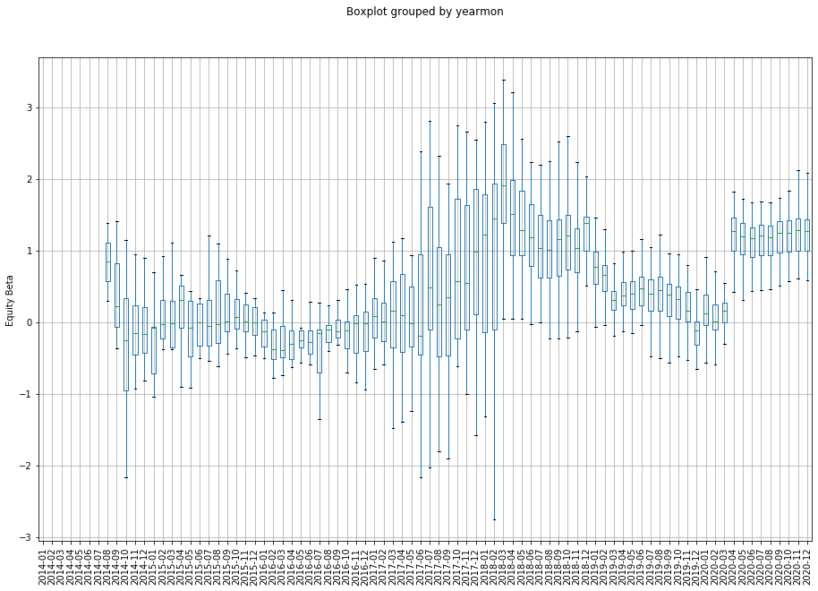
Alongside looking at simple cross-sectional averages of our factors across time, we also care about the distribution of these factors. We can use a simple boxplot to examine this. Key features to look for are changes in the spread of values in the IQR, as well as how far away the min/max values are from the mean. If you see large volatility in the factors, or sudden changes in the distribution, this could suggest that there’s potentially something wrong in your calculation, or the factor itself is very unstable and thus might not be suitable for investment.
Our first chart looks at the change in the beta for each coin against the S&P500. What’s interesting is the marked shift in beta that occured in April 2020, as well as the significant decline in spread that occurred in April 2018.
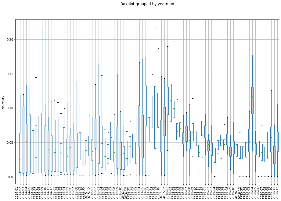
Our second charge look at return volatility, where we see the natural result of the very large spike in volatility that occurred in late 2017/early 2018. The behaviour of this spike is significantly different to the recent 2020 acceleration in BTC price. This suggests that there’s potentially a more orderly price increase going on, which may be suggestive of a more stable price behaviour.
Univariate portfolios
After studying the factors, the next step is to usually construct a portfolio. To do this, for your factor, on the portfolio rebalancing date, you sort based on your factor and then split all of your assets into $N$ number of groups. We use 3, due to the small number of assets. The typical approach is to use 5 or 10 portfolios. Within each portfolio, you can then calculate a portfolio return for each month. The standard approach is to use a value-weighted return (on market cap) or an equal-weighted return (simple average). In reality, your portfolio likely will be weighted differently (for example, optimised using mean-variance) so you would need to take this into account.
Now that you have returns for each of your portfolios, for each factor, for each month, you can study the average behaviour. The standard approach is to assume that you can go 100% long the “high” portfolio (i.e. portfolio associated with high values of your factor) and 100% short the “low” portfolio. This naturally has numerous problems, primarily the assumption that you can short everything in the “low” portfolio. However, it suffices as a theoretical representation of the possible validity of the factor in predicting returns. Dealing with implementation and feasibility is often left to industry, rather than academia.
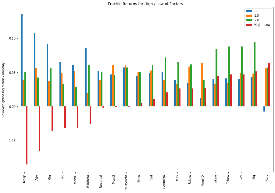
One common method of studying portfolios is to study the various factors within each portfolio. This highlights potential similarities in factors and expected characteristics. Here, we sort our portfolio on market cap and then study the factors.
We find several results:
- Low market cap is associated with highly illiquid assets, which also have the largest/smallest returns and tend to have higher levers of skewness.
- Interestingly, the cryptobeta is relatively similar across all market caps.
Typically, you would follow this approach for your “new” factor of interest, to examine how it related to existing factors.
| Low | Mid | High | |
|---|---|---|---|
| illiq | 12.4336 | 0.2182 | 0.0096 |
| skew | 0.0934 | 0.1519 | 0.0413 |
| kurt | 1.4823 | 1.5420 | 1.9720 |
| max | 0.1701 | 0.1510 | 0.1258 |
| min | -0.1557 | -0.1420 | -0.1240 |
| vol | 0.0745 | 0.0631 | 0.0523 |
| adv | 699,484.4725 | 2,364,494.7222 | 34,097,672.6168 |
| prc | -1.6425 | -0.7282 | 1.7107 |
| mcap | 16.7907 | 18.4369 | 21.0523 |
| equitybeta | 0.2769 | 0.5381 | 0.4723 |
| ivol | 1.2439 | 1.1108 | 0.9261 |
| iskew | 0.5959 | 0.5582 | 0.3027 |
| sskew | 16.4579 | 5.3209 | 8.8939 |
| tskew | 0.4138 | 0.4431 | 0.0825 |
| gold_beta | 0.6139 | 0.5050 | 0.3769 |
| cryptobeta | 0.9311 | 0.9060 | 0.9451 |
| mom_3 | -0.0890 | 0.0720 | 0.1091 |
| mom_6 | -0.1190 | 0.1622 | 0.2273 |
| mom_12 | -0.1919 | 0.3876 | 0.4364 |
| reversal | -0.0373 | 0.0040 | 0.0323 |
| monthly_rf | 0.0146 | -0.0286 | 0.0027 |
This chart shows the cumulative value-weighted log-returns associated with the long/short portfolios for each of our factors. In essence, it’s the cumulative returns associated with the factor if you had been able to construct a long/short portfolio.
What is particularly interesting here, is post 2018 the flatlining of almost every single factor. This is potentially suggestive of the market becoming incredibly saturated as investors piled in after the crash. There are many interpretations that could be explored, perhaps none of these are genuine pricing factors and it’s simply random noise, perhaps the underlying assets are far too volatile to draw any meaningful conclusions.
This highlights one of the primary problems with studying cryptocurrencies, we only have 6 years of good data, at best. It’s incredibly difficult to draw any meaningful results from such a small timeframe. A more fruitful area would be in examining tick-by-tick behaviour, where there is substantially more data to study.
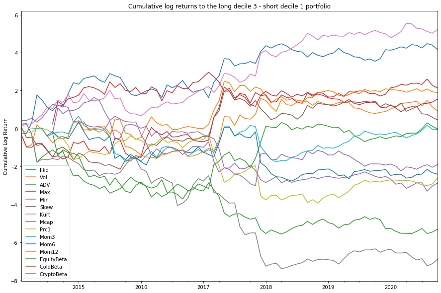
In summary, we find that there is a significant size/volume factor present, which produces significantly negative returns. On the positive side, factors that are anti-correlated with market cap produce positive excess returns. Interestingly, we find that standard momentum/reversal factors don’t produce any returns. This is likely because we use monthly frequency, and the behaviour of crypto might be simply too high frequency to capture any long-term momentum returns.
Another common technique in academic finance is to use Fama-Macbeth (1973) regressions to study the efficacy of factors in predicting future returns, in the presence of multiple factors. There are issues with this approach, such as assuming linearity, and having to deal with collinearity, but it serves as a commonly accepted approach to study factor behaviour.
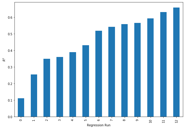
We run 13 regressions, where we incrementally add a factor into each regression specification.
This table shows the average coefficient associated with each factor, and a corresponding t-stat. The primary conclusion is that there’s no statistically significant factors which predict one-month forward returns. However, looking at the $R^2$ across each regression we run, we can see that we can indeed explain a large portion of the cross-sectional returns. This is potentially due to the very small dataset we’re working with. If we used a full set of coins, we would expect this $R^2$ value to drop significantly.
| variable | Mean | T-Stat |
|---|---|---|
| factor | ||
| max | -0.0169 | -0.9388 |
| iskew | -0.0140 | -1.1293 |
| illiq | -0.0139 | -1.0412 |
| min | -0.0071 | -0.7229 |
| alpha | -0.0025 | -1.1173 |
| ivol | -0.0025 | -1.1074 |
| cryptobeta | -0.0011 | -1.1304 |
| skew | -0.0009 | -1.0767 |
| reversal | -0.0004 | -0.4896 |
| equitybeta | -0.0001 | -1.1523 |
| sskew | -0.0000 | -1.1251 |
| adv | -0.0000 | -1.0430 |
| mcap | 0.0001 | 1.1284 |
| kurt | 0.0002 | 1.1011 |
| mom_12 | 0.0002 | 1.1306 |
| gold_beta | 0.0013 | 1.1163 |
| tskew | 0.0141 | 1.1294 |
| vol | 0.1056 | 1.0993 |