Exploration of Baseball Data

Supplied via: https://www.kaggle.com/timschutzyang/dataset1

import pandas as pd
import numpy as np
import matplotlib.pyplot as plt
import seaborn as sns

df = pd.read_csv("baseballdata.csv")
df.head()

	Unnamed: 0	Rk	Year	Tm	Lg	G	W	L	W.L.	...	R	RA	Attendance	BatAge	PAge	X.Bat	X.P	Top.Player	Managers	current
0	1	1	2016	Arizona Diamondbacks	NL West	162	69	93	0.426	...	752	890	2,036,216	26.7	26.4	50	29	J.Segura (5.7)	C.Hale (69-93)	Arizona Diamondbacks
1	2	2	2015	Arizona Diamondbacks	NL West	162	79	83	0.488	...	720	713	2,080,145	26.6	27.1	50	27	P.Goldschmidt (8.8)	C.Hale (79-83)	Arizona Diamondbacks
2	3	3	2014	Arizona Diamondbacks	NL West	162	64	98	0.395	...	615	742	2,073,730	27.6	28.0	52	25	P.Goldschmidt (4.5)	K.Gibson (63-96) and A.Trammell (1-2)	Arizona Diamondbacks
3	4	4	2013	Arizona Diamondbacks	NL West	162	81	81	0.500	...	685	695	2,134,895	28.1	27.6	44	23	P.Goldschmidt (7.1)	K.Gibson (81-81)	Arizona Diamondbacks
4	5	5	2012	Arizona Diamondbacks	NL West	162	81	81	0.500	...	734	688	2,177,617	28.3	27.4	48	23	A.Hill (5.0)	K.Gibson (81-81)	Arizona Diamondbacks

5 rows × 24 columns

df.count()

Unnamed: 0    2594
Rk            2594
Year          2594
Tm            2594
Lg            2594
G             2594
W             2594
L             2594
Ties          2594
W.L.          2594
pythW.L.      2594
Finish        2594
GB            2594
Playoffs       431
R             2594
RA            2594
Attendance    2520
BatAge        2594
PAge          2594
X.Bat         2594
X.P           2594
Top.Player    2594
Managers      2594
current       2594
dtype: int64

df.isnull().any()

Unnamed: 0    False
Rk            False
Year          False
Tm            False
Lg            False
G             False
W             False
L             False
Ties          False
W.L.          False
pythW.L.      False
Finish        False
GB            False
Playoffs       True
R             False
RA            False
Attendance     True
BatAge        False
PAge          False
X.Bat         False
X.P           False
Top.Player    False
Managers      False
current       False
dtype: bool

Data Cleaning

df["Date"] = pd.to_datetime(df["Year"].astype(str)+"-12-31")
df["Attendance"] = df["Attendance"].str.replace(",","").astype(float)
df["Manager"] = df["Managers"].str.split("((\([0-9]))", expand = True)[0]

Team/Manager Plots

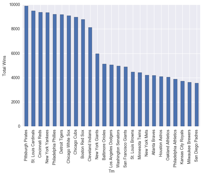
df.groupby("Tm").sum()["W"].sort_values(ascending=False)[0:25].plot(kind="bar")
plt.ylabel("Total Wins")
plt.show()

png

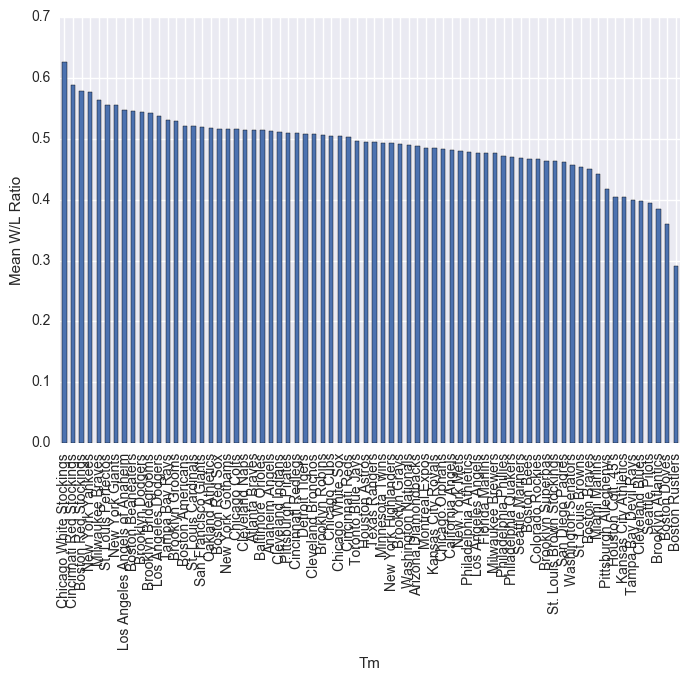
df.groupby("Tm").mean()["W.L."].sort_values(ascending=False).plot(kind="bar")
plt.ylabel("Mean W/L Ratio")
plt.show()

png

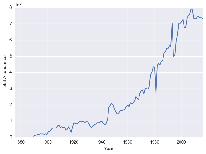
df.groupby("Year").sum()["Attendance"].plot()
plt.ylabel("Total Attendance")
plt.show()

png

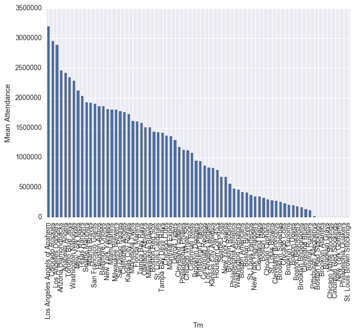
df.groupby("Tm").mean()["Attendance"].sort_values(ascending=False).plot(kind="bar")
plt.ylabel("Mean Attendance")
plt.show()

png

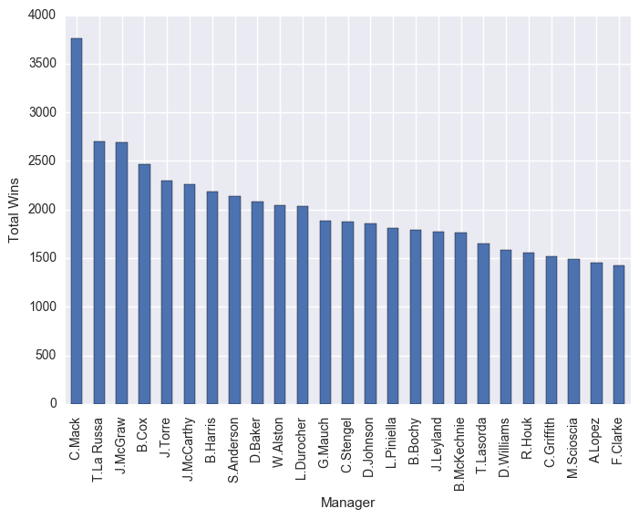
df.groupby("Manager").sum()["W"].sort_values(ascending=False)[0:25].plot(kind="bar")
plt.ylabel("Total Wins")
plt.show()

png

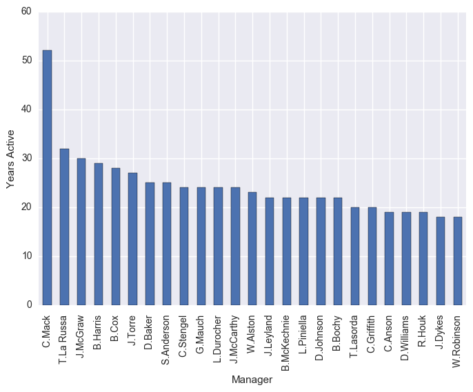
df.groupby("Manager").count()["Year"].sort_values(ascending=False)[0:25].plot(kind="bar")
plt.ylabel("Years Active")
plt.show()

png

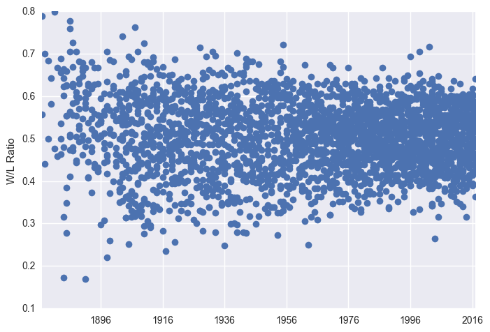
Variables Over Time

Here we plot a range of statistics over time, and look at some trends in them.

plt.plot_date(x = df["Date"], y = df["W.L."])
plt.ylabel("W/L Ratio")
plt.show()

png

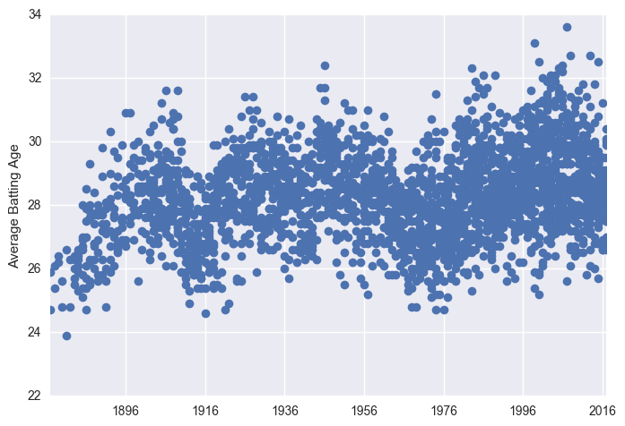
plt.plot_date(x = df["Date"], y = df["BatAge"])
plt.ylabel("Average Batting Age")
plt.show()

png

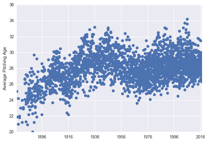
plt.plot_date(x = df["Date"], y = df["PAge"])
plt.ylabel("Average Pitching Age")
plt.show()

png

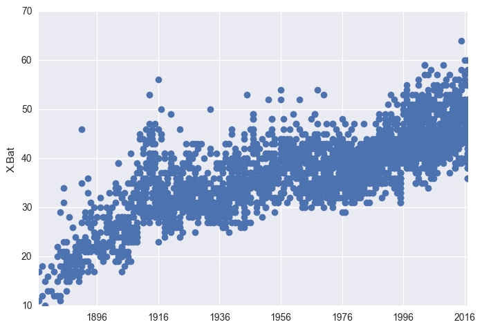
plt.plot_date(x = df["Date"], y = df["X.Bat"])
plt.ylabel("X.Bat") # not sure what this var is
plt.show()

png

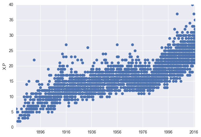
plt.plot_date(x = df["Date"], y = df["X.P"])
plt.ylabel("X.P") # not sure what this var is
plt.show()

png

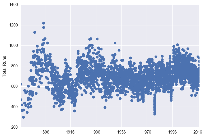
plt.plot_date(x = df["Date"], y = df["R"])
plt.ylabel("Total Runs")
plt.show()

png

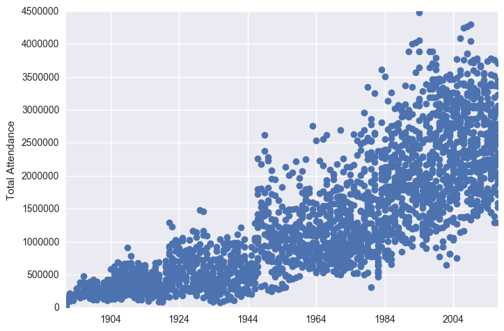
plt.plot_date(x = df["Date"], y = df["Attendance"])
plt.ylabel("Total Attendance")
plt.show()

png

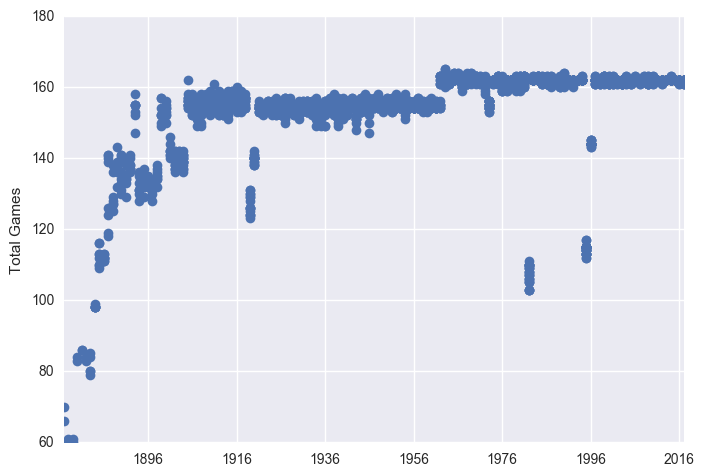
plt.plot_date(x = df["Date"], y = df["G"])
plt.ylabel("Total Games")
plt.show()

png

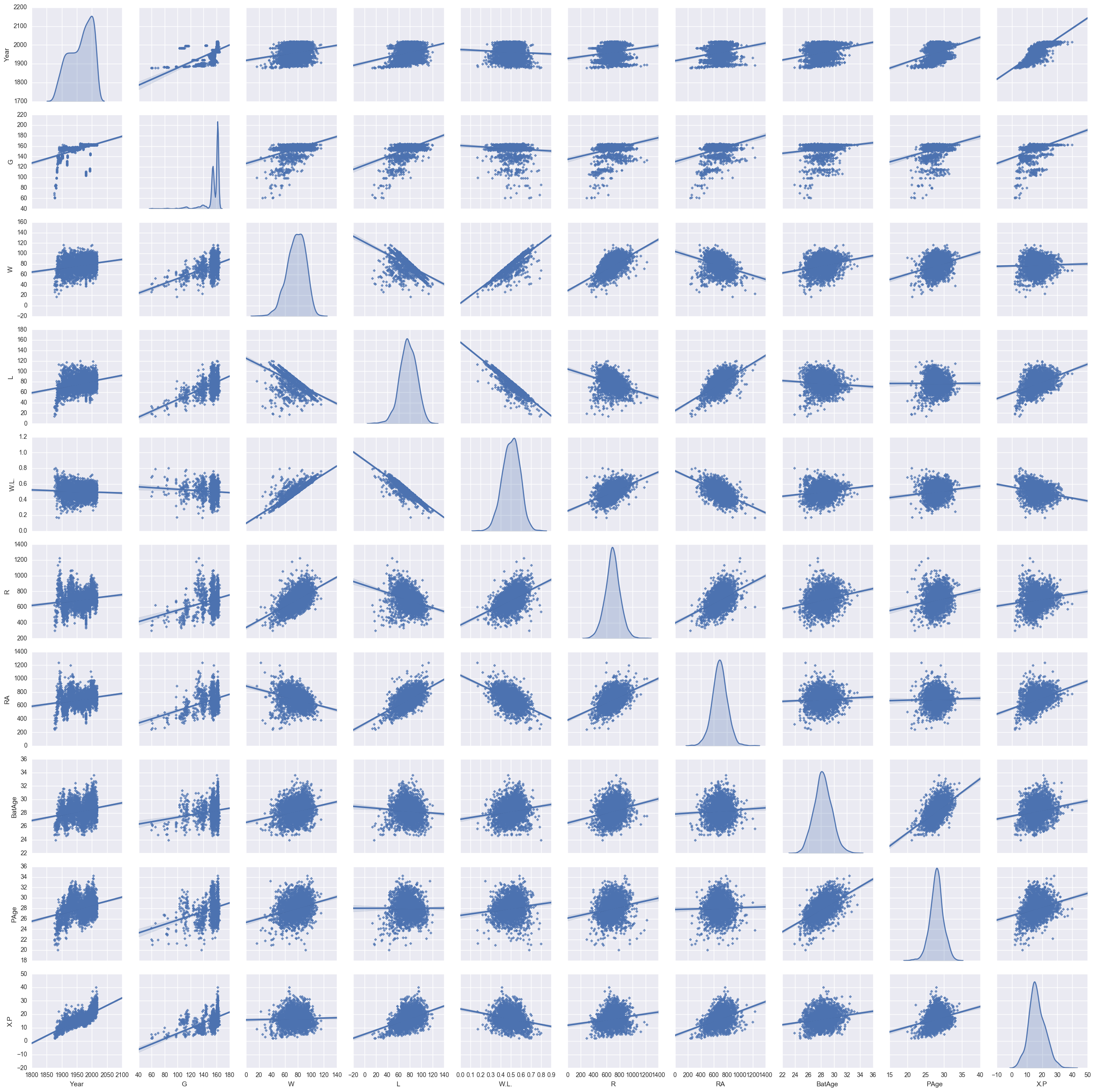
features = ["Year","G", "W", "L", "W.L.","R", "RA", "BatAge", "PAge", "X.P"]
sns.pairplot(df, vars = features, diag_kind = "kde", kind = "reg",
             markers = "+",
             diag_kws=dict(shade=True))
plt.show()

C:\Users\Clint_PC\Anaconda3\lib\site-packages\statsmodels\nonparametric\kdetools.py:20: VisibleDeprecationWarning: using a non-integer number instead of an integer will result in an error in the future
  y = X[:m/2+1] + np.r_[0,X[m/2+1:],0]*1j

png

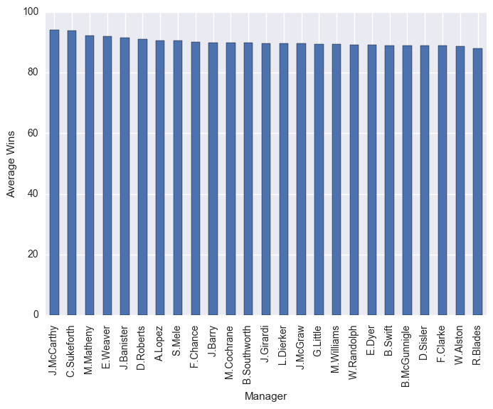
managers = df.groupby("Manager").mean()
managers["W"].sort_values(ascending=False)[0:25].plot(kind="bar")
plt.ylabel("Average Wins")
plt.show()

png

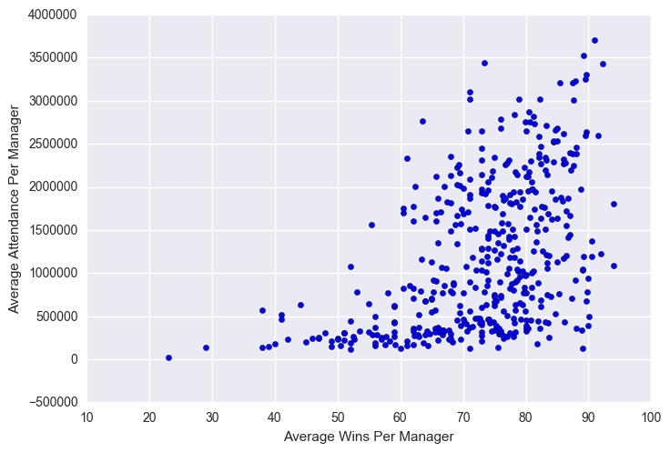
plt.scatter(x = managers["W"], y = managers["Attendance"])
plt.xlabel("Average Wins Per Manager")
plt.ylabel("Average Attendance Per Manager")
plt.show()

png

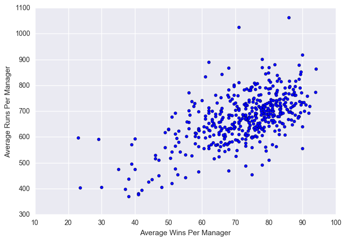
plt.scatter(x = managers["W"], y = managers["R"])
plt.xlabel("Average Wins Per Manager")
plt.ylabel("Average Runs Per Manager")
plt.show()

png