Investigation of Bank Failures
Data provided from Kaggle: https://www.kaggle.com/fdic/bank-failures
import numpy as np
import pandas as pd
import matplotlib.pyplot as plt
import seaborn as sns
df = pd.read_csv("bank-failures/banks.csv")
df.head()
df.count()
Financial Institution Number    2883
Institution Name                3484
Institution Type                3484
Charter Type                    3484
Headquarters                    3484
Failure Date                    3484
Insurance Fund                  3484
Certificate Number              2999
Transaction Type                3484
Total Deposits                  3484
Total Assets                    3333
Estimated Loss (2015)           2509
dtype: int64
Data Cleaning
df = df.join( df["Headquarters"].str.split(",", expand = True))
df["D/A"] = df["Total Deposits"]/df["Total Assets"]
df["Failure Date"] = pd.to_datetime(df["Failure Date"])
df = df.rename(columns = {0:"City", 1:"State", 2:"Del"})
df = df.drop("Del", 1)
df.count()
Financial Institution Number    2883
Institution Name                3484
Institution Type                3484
Charter Type                    3484
Headquarters                    3484
Failure Date                    3484
Insurance Fund                  3484
Certificate Number              2999
Transaction Type                3484
Total Deposits                  3484
Total Assets                    3333
Estimated Loss (2015)           2509
City                            3484
State                           3484
D/A                             3333
dtype: int64
Time Plots
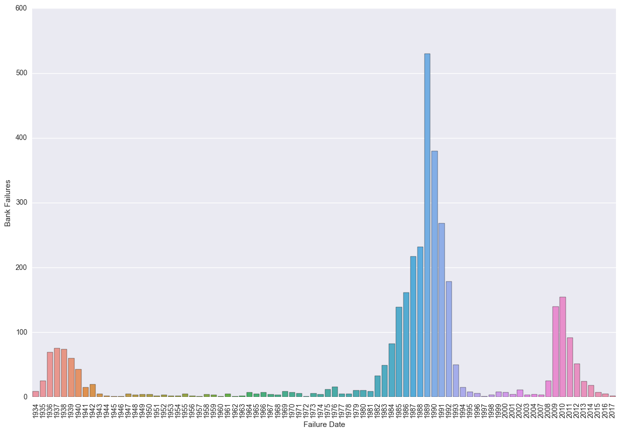
Not unexpectedly, we see the largest peaks in the lates 80’s and early 90’s corresponding to the Savings and Loan crisis, 2009/2010 corresponding to the GFC and the late 30’s with The Great Depression. What would be more interesting would be to look at the percentage failures of banks (to do.)
fails_by_year = df['Failure Date'].groupby([df["Failure Date"].dt.year]).agg('count')
plt.figure(figsize=(15,10))
sns.barplot(fails_by_year.index, fails_by_year)
plt.xticks(rotation="vertical")
plt.ylabel("Bank Failures")
plt.show()
Geographical Plots
df.groupby("State").count()["Failure Date"].sort_values(ascending=False)[0:25].plot(kind="bar")
plt.ylabel("Total Failures")
plt.show()
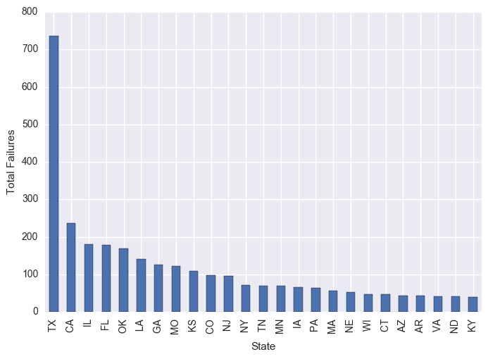
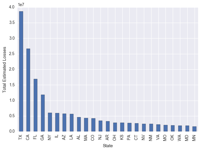
We see that TX has both the largest number of failures and the largest total estimated losses. Let’s see whose contributing to this.
df.groupby("State").sum()["Estimated Loss (2015)"].sort_values(ascending=False)[0:25].plot(kind="bar")
plt.ylabel("Total Estimated Losses")
plt.show()
df[df["State"] == " TX"].sort_values(by = "Estimated Loss (2015)", ascending = False)[0:10]
| Financial Institution Number | Institution Name | Institution Type | Charter Type | Headquarters | Failure Date | Insurance Fund | Certificate Number | Transaction Type | Total Deposits | Total Assets | Estimated Loss (2015) | City | State | D/A | |
|---|---|---|---|---|---|---|---|---|---|---|---|---|---|---|---|
| 1520 | 6938.0 | UNIVERSITY FEDERAL SAVINGS | SAVINGS ASSOCIATION | FEDERAL/STATE | HOUSTON, TX | 1989-02-14 | RTC | 30685.0 | ACQUISITION | 3776427 | 4480389.0 | 2177985.0 | HOUSTON | TX | 0.842879 |
| 1377 | 2846.0 | FIRST REPUBLICBANK-DALLAS, N.A. | COMMERCIAL BANK | FEDERAL | DALLAS, TX | 1988-07-29 | FDIC | 3165.0 | ACQUISITION | 7680063 | 17085655.0 | 2017459.0 | DALLAS | TX | 0.449504 |
| 2363 | 2124.0 | SAN JACINTO SAVINGS | SAVINGS ASSOCIATION | FEDERAL/STATE | HOUSTON, TX | 1990-11-30 | RTC | 31058.0 | ACQUISITION | 2894745 | 2869629.0 | 1700654.0 | HOUSTON | TX | 1.008752 |
| 1506 | 7070.0 | GILL SA | SAVINGS ASSOCIATION | FEDERAL/STATE | SAN ANTONIO, TX | 1989-02-07 | RTC | 31503.0 | ACQUISITION | 1448432 | 1207294.0 | 1659803.0 | SAN ANTONIO | TX | 1.199734 |
| 1618 | 7335.0 | COMMONWEALTH SAVINGS ASSOC. | SAVINGS ASSOCIATION | FEDERAL/STATE | HOUSTON, TX | 1989-03-09 | RTC | 31896.0 | TRANSFER | 1608452 | 1647893.0 | 1613353.0 | HOUSTON | TX | 0.976066 |
| 1714 | 2985.0 | MBANK DALLAS, NATIONAL ASSOCIATION | COMMERCIAL BANK | FEDERAL | DALLAS, TX | 1989-03-28 | FDIC | 3163.0 | ACQUISITION | 4033803 | 6556056.0 | 1610809.0 | DALLAS | TX | 0.615279 |
| 1517 | 6952.0 | BRIGHT BANC | SAVINGS ASSOCIATION | FEDERAL/STATE | DALLAS, TX | 1989-02-10 | RTC | 31095.0 | ACQUISITION | 3004443 | 4388466.0 | 1307798.0 | DALLAS | TX | 0.684623 |
| 1823 | 2100.0 | VICTORIA SA | SAVINGS ASSOCIATION | FEDERAL/STATE | SAN ANTONIO, TX | 1989-06-29 | RTC | 29378.0 | PAYOUT | 855717 | 882849.0 | 968972.0 | SAN ANTONIO | TX | 0.969268 |
| 1627 | 2104.0 | BANCPLUS SAVINGS ASSOCIATION | SAVINGS ASSOCIATION | FEDERAL/STATE | PASADENA, TX | 1989-03-09 | RTC | 31128.0 | ACQUISITION | 923026 | 751461.0 | 964160.0 | PASADENA | TX | 1.228309 |
| 1619 | 7429.0 | BENJAMIN FRANKLIN SA | SAVINGS ASSOCIATION | FEDERAL/STATE | HOUSTON, TX | 1989-03-09 | RTC | 30761.0 | ACQUISITION | 2004722 | 2641392.0 | 882240.0 | HOUSTON | TX | 0.758964 |
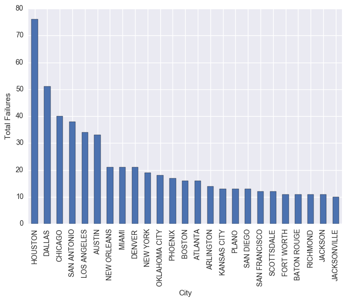
df.groupby("City").count()["Failure Date"].sort_values(ascending=False)[0:25].plot(kind="bar")
plt.ylabel("Total Failures")
plt.show()
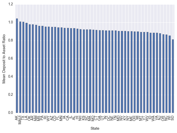
df.groupby("State").mean()["D/A"].sort_values(ascending=False)[0:50].plot(kind="bar")
plt.ylabel("Mean Deposit to Asset Ratio")
plt.show()
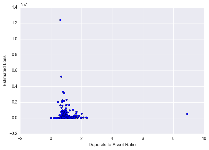
Deposit to Assets
Ignoring the possibility that this is not real and hence not inflation adjusted. Interesting to see whether there is any relationship between D/A and the losses suffered. It looks like there is no strong correlation at all, which would indicate that it’s not necessarily a mismanagement of deposits/assets which have driven bank failures, but other factors. Typically it’s liquidity which brings the banks down, after sustaining a systemic asset shock (housing/mortgage exposures in the GFC).
plt.scatter(x = df["D/A"], y = df["Estimated Loss (2015)"])
plt.xlabel("Deposits to Asset Ratio")
plt.ylabel("Estimated Loss")
plt.show()
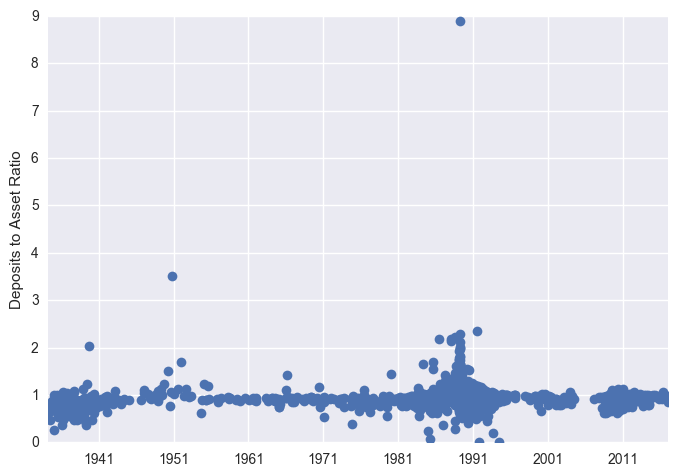
plt.plot_date(x = df["Failure Date"], y = df["D/A"])
plt.ylabel("Deposits to Asset Ratio")
plt.show()