Analysis of NRL Data
Extension of work from Fisadev (utility functions used are derived from previous NB) but utilising Keras and NRL data. Still a work in progress..
1. Libraries
import pandas as pd
import numpy as np
import matplotlib.pyplot as plt
import seaborn as sns
import utils

# Scikit-Learn deprecation warnings, turn off.
import warnings
warnings.filterwarnings("ignore", category=DeprecationWarning)
2. Data IO
We’ll be using historical NRL data obtained from: http://www.aussportsbetting.com/data/ Which comes with the disclaimer “The following data set may contain errors. It is a condition of use that you do not rely upon the information provided in this spreadsheet when making wagering decisions. Please verify everything for yourself.”
We’ll also use a dataset which shows the top 4 places in each year of the competition since 2009. Some things to look out for in the data include:
- Multiple names for the same team
- Draws
nrl_raw = pd.read_excel("nrl.xlsx", header = 1)
nrl_winners = pd.read_csv("nrl_raw_winners.csv")
3. Data Cleaning
Here we’re going to clean the data into a more basic format, and include only the data we deem relevant for analysis.
nrl_raw.head(5)
| Date | Kick-off (local) | Home Team | Away Team | Home Score | Away Score | Play Off Game? | Over Time? | Home Odds | Draw Odds | ... | Total Score Close | Total Score Over Open | Total Score Over Min | Total Score Over Max | Total Score Over Close | Total Score Under Open | Total Score Under Min | Total Score Under Max | Total Score Under Close | Notes | |
|---|---|---|---|---|---|---|---|---|---|---|---|---|---|---|---|---|---|---|---|---|---|
| 0 | 2016-10-02 | 19:15:00 | Melbourne Storm | Cronulla Sharks | 12 | 14 | Y | NaN | 1.86 | 17.94 | ... | 34.5 | 1.925 | 1.854 | 1.952 | 1.943 | 1.925 | 1.833 | 1.925 | 1.909 | NaN |
| 1 | 2016-09-24 | 19:40:00 | Melbourne Storm | Canberra Raiders | 14 | 12 | Y | NaN | 1.42 | 20.72 | ... | 36.0 | 1.925 | 1.862 | 2.050 | 1.862 | 1.925 | 1.925 | 1.925 | 1.990 | NaN |
| 2 | 2016-09-23 | 19:55:00 | Cronulla Sharks | North QLD Cowboys | 32 | 20 | Y | NaN | 2.02 | 18.76 | ... | 36.5 | 1.925 | 1.917 | 1.980 | 1.970 | 1.925 | 1.877 | 1.934 | 1.884 | NaN |
| 3 | 2016-09-17 | 19:40:00 | Canberra Raiders | Penrith Panthers | 22 | 12 | Y | NaN | 1.66 | 19.23 | ... | 42.5 | 1.961 | 1.961 | 1.990 | 1.990 | 1.892 | 1.892 | 1.862 | 1.862 | NaN |
| 4 | 2016-09-16 | 19:55:00 | North QLD Cowboys | Brisbane Broncos | 26 | 20 | Y | Y | 1.49 | 20.97 | ... | 38.0 | 1.925 | 1.925 | 1.970 | 1.943 | 1.925 | 1.925 | 2.000 | 1.909 | NaN |
5 rows × 49 columns
nrl_df = pd.DataFrame(columns = ["year", "team1", "score1", "score2", "team2"])
nrl_df.year = pd.to_datetime(nrl_raw.Date)
nrl_df.year = nrl_df.year.apply(lambda x: x.year)
nrl_df.team1 = nrl_raw["Home Team"]
nrl_df.score1 = nrl_raw["Home Score"]
nrl_df.score2 = nrl_raw["Away Score"]
nrl_df.team2 = nrl_raw["Away Team"]
print(nrl_df.head(5))
print(nrl_winners.head(5))
   year              team1  score1  score2              team2
0  2016    Melbourne Storm      12      14    Cronulla Sharks
1  2016    Melbourne Storm      14      12   Canberra Raiders
2  2016    Cronulla Sharks      32      20  North QLD Cowboys
3  2016   Canberra Raiders      22      12   Penrith Panthers
4  2016  North QLD Cowboys      26      20   Brisbane Broncos
   id  year  position               team
0   0  2010         1  St George Dragons
1   1  2010         2   Penrith Panthers
2   2  2010         3       Wests Tigers
3   3  2010         4  Gold Coast Titans
4   4  2009         1  St George Dragons
print(np.unique(set(nrl_df.team1.unique()).union(nrl_df.team2.unique())))
print(np.unique(nrl_winners.team))
[ {'Wests Tigers', 'Manly-Warringah Sea Eagles', 'Canterbury-Bankstown Bulldogs', 'South Sydney Rabbitohs', 'Newcastle Knights', 'Melbourne Storm', 'Manly Sea Eagles', 'St. George Illawarra Dragons', 'Cronulla Sharks', 'North Queensland Cowboys', 'Gold Coast Titans', 'Sydney Roosters', 'Canterbury Bulldogs', 'Brisbane Broncos', 'Parramatta Eels', 'St George Dragons', 'Penrith Panthers', 'New Zealand Warriors', 'North QLD Cowboys', 'Canberra Raiders', 'Cronulla-Sutherland Sharks'}]
['Brisbane Broncos' 'Canberra Raiders' 'Canterbury Bulldogs'
 'Canterbury Bulldogs Bulldogs' 'Cronulla Sharks' 'Gold Coast Titans'
 'Manly Sea Eagles' 'Melbourne Storm' 'North Queensland' 'Penrith Panthers'
 'South Sydney Rabbitohs' 'St George Dragons' 'Sydney Roosters'
 'Wests Tigers']
We clearly see that there are some name double-ups both within the names and between the two datasets we’re using:
- Cronulla Sharks and Cronulla-Sutherland Sharks
- St. George Illawarra Dragons and St George Dragons
So we’ll have to deal with this.
def replace_all_keys(s, dict):
    for i, j in dict.items():
        s = s.replace(i, j)
    return s

replacement_key = {"St. George Illawarra Dragons" : "St George Dragons",
                    "Cronulla-Sutherland Sharks" : "Cronulla Sharks",
                  "Manly-Warringah Sea Eagles" : "Manly Sea Eagles",
                  "Canterbury-Bankstown Bulldogs" : "Canterbury Bulldogs",
                  "North Queensland Cowboys" : "North QLD Cowboys"}

nrl_df = nrl_df.apply(lambda x: replace_all_keys(x, replacement_key))
print(np.unique(set(nrl_df.team1.unique()).union(nrl_df.team2.unique())))

replacement_key_2 = {"North Queensland" : "North QLD Cowboys",
                    "Canterbury Bulldogs Bulldogs" : "Canterbury Bulldogs"}

nrl_winners = nrl_winners.apply(lambda x: replace_all_keys(x, replacement_key_2))
print(np.unique(nrl_winners.team))
[ {'Wests Tigers', 'South Sydney Rabbitohs', 'Newcastle Knights', 'Melbourne Storm', 'Manly Sea Eagles', 'Cronulla Sharks', 'Gold Coast Titans', 'Sydney Roosters', 'Canterbury Bulldogs', 'Brisbane Broncos', 'Parramatta Eels', 'St George Dragons', 'Penrith Panthers', 'New Zealand Warriors', 'North QLD Cowboys', 'Canberra Raiders'}]
['Brisbane Broncos' 'Canberra Raiders' 'Canterbury Bulldogs'
 'Cronulla Sharks' 'Gold Coast Titans' 'Manly Sea Eagles' 'Melbourne Storm'
 'North QLD Cowboys' 'Penrith Panthers' 'South Sydney Rabbitohs'
 'St George Dragons' 'Sydney Roosters' 'Wests Tigers']
4. Basic Exploration
We’re going to utilise some utility functions to extra out relevant information on the dataset. These functions allow us to derive out some basic match statistics.
def get_matches(with_team_stats=False):
    """Create a dataframe with matches info."""
    matches = nrl_df

    def winner(x):
        if x > 0:
            return 1
        elif x < 0:
            return 2
        else:
            return 0

    matches['score_diff'] = matches['score1'] - matches['score2']
    matches['winner'] = matches['score_diff']
    matches['winner'] = matches['winner'].map(winner)

    if with_team_stats:
        stats = get_team_stats()
        matches = matches.join(stats, on='team1')\
                         .join(stats, on='team2', rsuffix='_2')

    return matches

def get_team_stats():
    """Create a dataframe with useful stats for each team."""
    matches = get_matches()
    winners = nrl_winners

    # Find the set of all unique teams and initialise a dataframe to hold the stats we are going to calculate.
    teams = set(matches.team1.unique()).union(matches.team2.unique())
    stats = pd.DataFrame(list(teams), columns=['team'])
    stats = stats.set_index('team')

    # Iterate over each team and calculate the following statistics:
    # - Matches Won (%), Ratio of Points Scored/Points Conceded,
    # - Matches Lost, Yearly Podium Score
    for team in teams:
        team_matches = matches[(matches.team1 == team) | (matches.team2 == team)]
        stats.loc[team, 'matches_played'] = len(team_matches)

        # wins where the team was  the home side (team1)
        wins1 = team_matches[(team_matches.team1 == team) & (team_matches.score1 > team_matches.score2)]
        # wins where the team was  the away side (team2)
        wins2 = team_matches[(team_matches.team2 == team) & (team_matches.score2 > team_matches.score1)]

        stats.loc[team, "draws"] = len(team_matches[(team_matches.team1 == team) & (team_matches.score2 == team_matches.score1)]) + len(team_matches[(team_matches.team1 == team) & (team_matches.score2 == team_matches.score1)])

        stats.loc[team, "points_scored"] = sum(matches[matches.team1 == team].iloc[:,2]) + sum( matches[matches.team2 == team].iloc[:,3] )

        stats.loc[team, "points_conceded"] = sum(matches[matches.team1 == team].iloc[:,3]) + sum( matches[matches.team2 == team].iloc[:,2])
        stats.loc[team, 'matches_won'] = len(wins1) + len(wins2)
        stats.loc[team, 'years_played'] = len(team_matches.year.unique())

        # Map in the teams that have placed in the top 4, and then give them a weighting.
        team_podiums = winners[winners.team == team]
        to_score = lambda position: 2 ** (5 - position)  # better position -> more score, exponential
        stats.loc[team, 'podium_score'] = team_podiums.position.map(to_score).sum()

    stats['matches_won_percent'] = stats['matches_won'] / stats['matches_played'] * 100.0
    stats['scored/conceded'] = stats["points_scored"] / stats["points_conceded"]
    stats["losses"] = stats["matches_played"] - stats["matches_won"] - stats["draws"]
    stats['podium_score_yearly'] = stats['podium_score'] / stats['years_played']

    return stats
matches = get_matches()
stats = get_team_stats()
stats["matches_won_percent"].sort_values(ascending=False).plot(kind="bar")
plt.ylabel("Matches Won (%)")
plt.show()
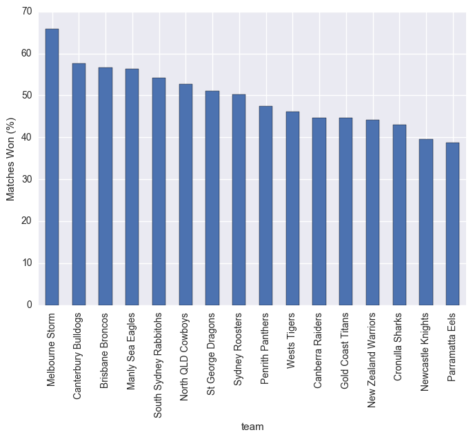
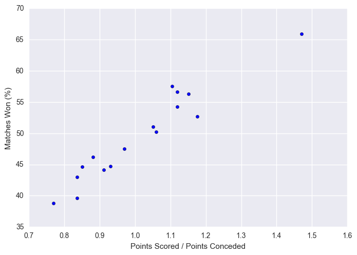
Not unexpectedly, higher points scored to points conceded results in a higher matches won %. What is interesting though is the quite linear structure here, could be useful in prediction.
plt.scatter(x = stats["scored/conceded"], y = stats["matches_won_percent"])
plt.xlabel("Points Scored / Points Conceded")
plt.ylabel("Matches Won (%)")
plt.show()
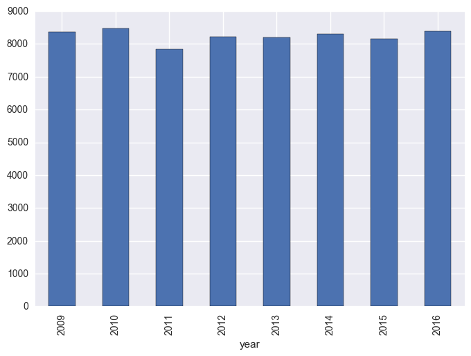
The below shows that there isn’t any large trend in points scored per season, which would be expected for a fairly mature competition.
matches["total_scored"] = matches["score1"] + matches["score2"]
matches.groupby("year").sum()["total_scored"].plot(kind="bar")
plt.show()
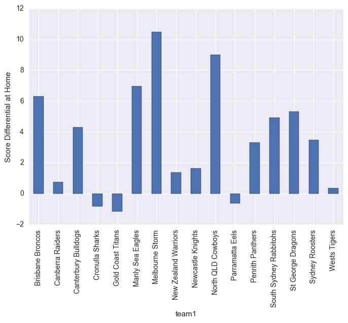
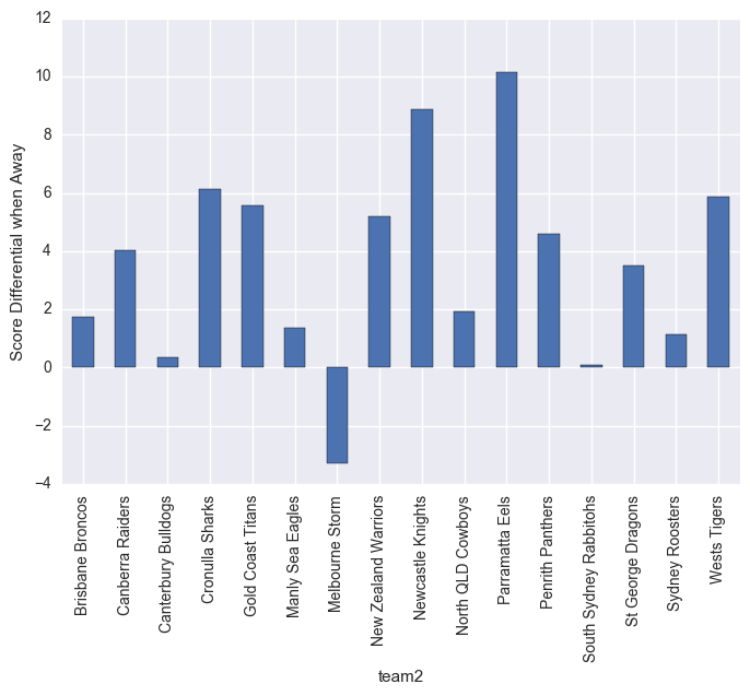
What the below graphs show are the point differentials. Clearly Melbourn Storm struggle on the road, but dominate at home. Leading into the Melbourn Storm home ground guru.
matches.groupby("team1").mean()["score_diff"].plot(kind="bar")
plt.ylabel("Score Differential at Home")
plt.show()
matches.groupby("team2").mean()["score_diff"].plot(kind="bar")
plt.ylabel("Score Differential when Away")
plt.show()
5. Prediction Definition
Given our previous indication, we’ll now seek to apply some very basic, rudimentary machine learning techniques to see if we can beat a coin-flip at guessing the winner of a match.
def extract_samples(matches, origin_features, result_feature):
    inputs = [tuple(matches.loc[i, feature] for feature in origin_features) for i in matches.index]
    outputs = tuple(matches[result_feature].values)

    assert len(inputs) == len(outputs)

    return inputs, outputs
from sklearn.preprocessing import StandardScaler

def normalize(array):
    scaler = StandardScaler()
    array = scaler.fit_transform(array)

    return scaler, array
from random import random

def split_samples(inputs, outputs, percent=0.66):
    assert len(inputs) == len(outputs)

    inputs1 = []
    inputs2 = []
    outputs1 = []
    outputs2 = []

    for i, inputs_row in enumerate(inputs):
        if random() < percent:
            input_to = inputs1
            output_to = outputs1
        else:
            input_to = inputs2
            output_to = outputs2

        input_to.append(inputs_row)
        output_to.append(outputs[i])

    return inputs1, outputs1, inputs2, outputs2
input_features = ["year",
                  "matches_won_percent",
                  "podium_score_yearly",
                  "scored/conceded",
                  "matches_won_percent_2",
                  "podium_score_yearly_2",
                  "scored/conceded_2"]

output_feature = "winner"
matches = get_matches(with_team_stats=True)
inputs, outputs = extract_samples(matches, input_features, output_feature)
normalizer, inputs = normalize(inputs)

train_inputs, train_outputs, test_inputs, test_outputs = split_samples(inputs, outputs)
6. Basic Models
from sklearn.svm import SVC
from sklearn.linear_model import LogisticRegression
from sklearn.ensemble import RandomForestClassifier
from sklearn.model_selection import KFold, cross_val_score
k_fold = KFold(n_splits = 10)
clf = SVC()
clf.fit(train_inputs, train_outputs)
print("SVC Score: ",clf.score(test_inputs, test_outputs))

clf_forest = RandomForestClassifier(n_estimators=100)
clf_forest.fit(train_inputs, train_outputs)
print("Random Forest Score: ", clf_forest.score(test_inputs, test_outputs))

clf_logistic = LogisticRegression()
clf_logistic.fit(train_inputs, train_outputs)
print("Logistic Score: ", clf_logistic.score(test_inputs, test_outputs))
SVC Score:  0.612284069098
Random Forest Score:  0.57773512476
Logistic Score:  0.625719769674
We see that our prediction model doesn’t do that well, only just beating out a 50% probability. This premise is likely falling out from the lack of data available and the relatively small sample size being used.
7. Neural Nets
We can also explore the use of Keras here. We will use a very basic approach and give some demonstrative examples of how to apply Keras to this type of data. We’ll use a variety of basictechniques to demonstrate a basic Keras workflow with cross-validation.
from keras.models import Sequential
from keras.layers.core import Dense, Dropout, Activation
from keras.optimizers import RMSprop, SGD
from keras.utils import np_utils
from keras.utils.np_utils import to_categorical
from sklearn.model_selection import StratifiedKFold
X = np.array(inputs)
y = np.array(outputs).astype(float)
y[y == 2] = 0 # We treat 2 as a loss, 1 as a win. Normalise this so that 0 = loss, 1 = win.

kfold = StratifiedKFold(n_splits=10) # Kfold cross-validation
cvscores = [] # A store of cross-validation scores for each iteration of kfold
history = [] # A store of the keras history
for train, test in kfold.split(X, y):

  # Create sequential model which is basically a stack of linear neural layers.
    model = Sequential()
    model.add(Dense(12, activation='relu',input_dim=len(input_features) ))
    model.add(Dense(8, activation='relu'))
    model.add(Dense(1, activation='sigmoid'))

    # Compile model using stochastic gradient descent optimiser and binary crossentropy loss scoring.
    opt = SGD(lr=0.001)
    model.compile(loss = "binary_crossentropy", optimizer = opt, metrics = ["accuracy"])

    # Fit the model to training data
    history.append(model.fit(X[train], y[train], nb_epoch=150, batch_size=128, verbose=0))

    # Evaluate model against testing data
    scores = model.evaluate(X[test], y[test], verbose=0)
    print("%s: %.2f%%" % (model.metrics_names[1], scores[1]*100))
    cvscores.append(scores[1] * 100)
acc: 49.07%
acc: 57.14%
acc: 56.52%
acc: 53.42%
acc: 58.39%
acc: 58.39%
acc: 55.28%
acc: 50.31%
acc: 58.39%
acc: 59.75%
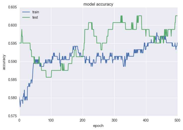
As expected, the results aren’t significantly improved on what we obtained with SVC and RF. Rather, we see that we typically see results in the range of 50-60%. Using this validation, we can now fit a model and draw some conclusions. Keras Documentation is quite handy…
history = model.fit(X, y, validation_split=0.33, nb_epoch=500, batch_size=128, verbose=0)
# Plot the accuracy of the train/test splits for each epoch.
plt.plot(history.history['acc'])
plt.plot(history.history['val_acc'])
plt.title('Model Accuracy')
plt.ylabel('Accuracy')
plt.xlabel('Epoch')
plt.legend(['train', 'test'], loc='upper left')
plt.show()
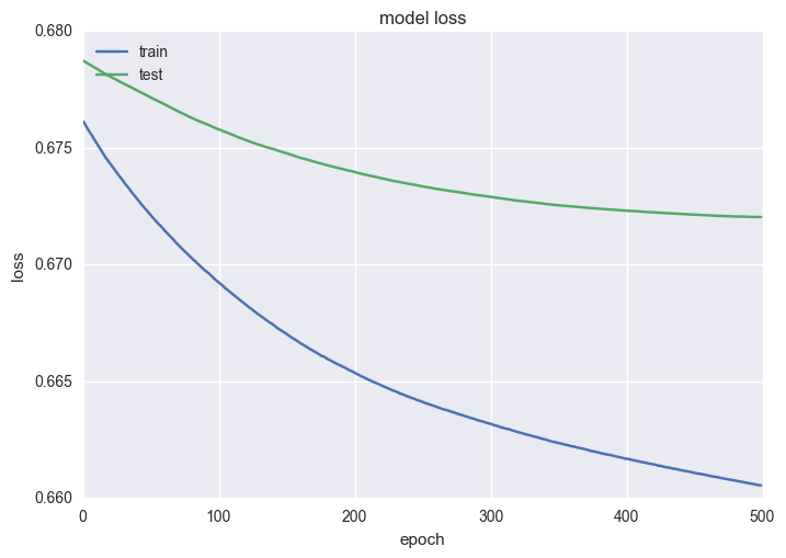
# Plot the loss of the train/test splits for each epoch
plt.plot(history.history['loss'])
plt.plot(history.history['val_loss'])
plt.title('Model Loss')
plt.ylabel('Loss')
plt.xlabel('Epoch')
plt.legend(['train', 'test'], loc='upper left')
plt.show()
model.summary()
____________________________________________________________________________________________________
Layer (type)                     Output Shape          Param #     Connected to
====================================================================================================
dense_289 (Dense)                (None, 12)            96          dense_input_97[0][0]
____________________________________________________________________________________________________
dense_290 (Dense)                (None, 8)             104         dense_289[0][0]
____________________________________________________________________________________________________
dense_291 (Dense)                (None, 1)             9           dense_290[0][0]
====================================================================================================
Total params: 209
Trainable params: 209
Non-trainable params: 0
____________________________________________________________________________________________________
8. Application to Prediction
def predict(year, team1, team2):
    inputs = []

    for feature in input_features:
        from_team_2 = '_2' in feature
        feature = feature.replace('_2', '')

        if feature in stats.columns.values:
            team = team2 if from_team_2 else team1
            value = stats.loc[team, feature]
        elif feature == 'year':
            value = year
        else:
            raise ValueError("Don't know where to get feature: " + feature)

        inputs.append(value)

    inputs = np.array([normalizer.transform(inputs)])
    result = model.predict(inputs)

    if result == 0.5:
        return 'tie'
    elif result > 0.5:
        return team1
    elif result < 0.5:
        return team2
    else:
        return "Unknown result: " + str(result)

print(predict(2013,"Cronulla Sharks", "Melbourne Storm"))
print(predict(2015, "Penrith Panthers", "Sydney Roosters"))
Melbourne Storm
Sydney Roosters
10. Extra Areas to Explore
It’s obvious that the implementations above are fairly basic, and are mainly just for showing how to apply the techniques rather than making super accurate predictions. There are many extra areas to explore, particularly around feature analysis and understanding of what features would actually drive predictions. We could perhaps incorporate things like:
- points scored ratios
- average point differentials
- number of representative level players etc.
The largest gains would probably come from incorporating some of the betting statistics which are available, based on head-to-head odds as well as significantly improving the quality of the data, perhaps expanding into player level data for each team.