Financial Data Scraping and Analysis - Fundamentals and Prices
There’s a treasure trove of financial data across the internet, but the two key ones that most people are interested in initially are fundamentals and pricing data. Pricing data (not live/tick-by-tick) is extremely easy to acquire from sources like Google Finance and Yahoo Finance API’s, whilst fundamental data is slightly more difficult as it’s often embedded into HTML tables and can’t be directly retrieved.
We’ll explore some different methods for retrieving data from the web, storing data into a MySQL database and then the subseqent retrieval and analysis of the data. All the data and commentary here is purely out of personal interest and is in no way financial advice.
MySQL Server
Before we do anything else, we should setup our MySQL server and two databases for our fundamental data and pricing data. Setting up the server is fairly straightforward and there’s a decent tutorial, check it here.
Once the database is up and running, it’ll give you a nice consistent method for storing data, as well as being able to retrieve it easily.
Scraping Pricing/Securities Data
Full Database Way
There are several tutorials on the web, the one from Quantstart is particularly good as they use SQL in it. With a slight adjustment, we can retrieve S&P data. I’ve added a function below which we can use to pull ASX200 data under the same Quantstart implementation.
def obtain_asx200():
    """Download and parse the Wikipedia list of ASX200
       Returns a list of tuples for to add to MySQL."""

  # Use libxml to download the list of S&P500 companies and obtain the symbol table
    now = datetime.utcnow()
    url = "http://www.asx200list.com/wp-content/uploads/csv/20170401-asx200.csv"
    s = requests.get(url).content
    df = pd.read_csv(io.StringIO(s.decode('utf-8')))
    df.columns = df.iloc[0]
    df = df.iloc[1:-1, 0:4]
    symbols = []
    for index, row in df.iterrows():
        symbols.append((row["Code"], 'stock', row["Company"], row["Sector"], 'AUD', now, now))

    return symbols
Simple Way to Scrape Financial Pricing Data
If you don’t want to go down the SQL path, and would prefer to keep a unified database in a store like HDF5 or a Pickel, there’s a good tutorial from The Algo Engineer here which I’ve adjusted slightly.
from pandas_datareader import data
from datetime import datetime
import pandas as pd
import requests
import io
from bs4 import BeautifulSoup
import pickle

def update_sp500_list():
    """ Downloads list of S&P500 companeis from Wikipedia.
    Returns a dictionary of sectors and tickers within each sector.
    """

    url = "http://en.wikipedia.org/wiki/List_of_S%26P_500_companies"
    hdr = {"User-Agent": "Mozilla/5.0"}
    request = urllib.request.Request(url, headers = hdr)
    page = urllib.request.urlopen(request)
    soup = BeautifulSoup(page)

    table = soup.find("table", {"class": "wikitable sortable"})
    sector_tickers = dict()
    for row in table.findAll("tr"):
        col = row.findAll("td")
        if len(col) > 0:
            # You can extract more data here from the Wikitable if you like, it has addresses, GICS subsectors etc
            sector = str(col[3].string.strip()).lower().replace(" ", "_")
            ticker = str(col[0].string.strip())
            if sector not in sector_tickers:
                sector_tickers[sector] = list()
            sector_tickers[sector].append(ticker)
    return sector_tickers


def get_ohlc_data(tickers, start, end):
    """ Download ticker data from yahoo-finance.

    Returns a multilevel dictionary with ticker data for each sector.
    """
    sector_data = {}
    for sector, tickers in tickers.items():
        print("Downloading sector: " + sector)
        tmp_data = data.DataReader(tickers, "yahoo", start, end)

        for item in ["Open", "High", "Low"]:
            tmp_data[item] = tmp_data[item] * tmp_data["Adj Close"] / tmp_data["Close"]
            tmp_data.rename(items = {"Open": "open",
                                     "High": "high",
                                     "Low": "low",
                                     "Adj Close": "close",
                                     "Volume": "volume"})

        #Add technical indicators if you please
        #tmp_data["MA"] = MA(tmp_data, 100, "Adj Close")
        #tmp_data["MOM"] = MOM(tmp_data, 100, "Adj Close")
        tmp_data.drop(["Close"], inplace = True)
        sector_data[sector] = tmp_data
    print("Finished.")
    return sector_data
The above script should run fairly seamlessly, you can then store/deal with your data however you like (HDF5, pickle, csv, etc.). I’ve chosen to use a basic pickling structure, and I’ll show some examples of data you can pull out. A dictionary structure is used, where each sector corresponds to a key, and within each sector the datafield we want corresponds to another key. So our structure is:
- Sector
- Field (Open, High, Low, Adj. Close Volume)
- Ticker time-series
start = datetime(1990,1,1)
end = datetime.utcnow()
path = "path/to/data/"
read_or_write = 0 # Flag based on whether we want to update our data or just read from disc.

if(read_or_write):
    sector_tickers = update_sp500_list() #Pull current ASX200/SP500 tickers
    sector_ohlc = get_ohlc_data(sector_tickers, start, end) #Pull yahoo fin data
    pickle.dump(sector_ohlc, open("sector_data.p", "wb"))
else:
    sector_ohlc = pickle.load(open(path, "rb"))

print("Sectors Obtained: " ,sector_ohlc.keys())
Sectors Obtained: dict_keys(['health_care', 'financials', 'consumer_discretionary', 'consumer_staples', 'industrials', 'information_technology', 'materials', 'real_estate', 'energy', 'utilities', 'telecommunications_services'])
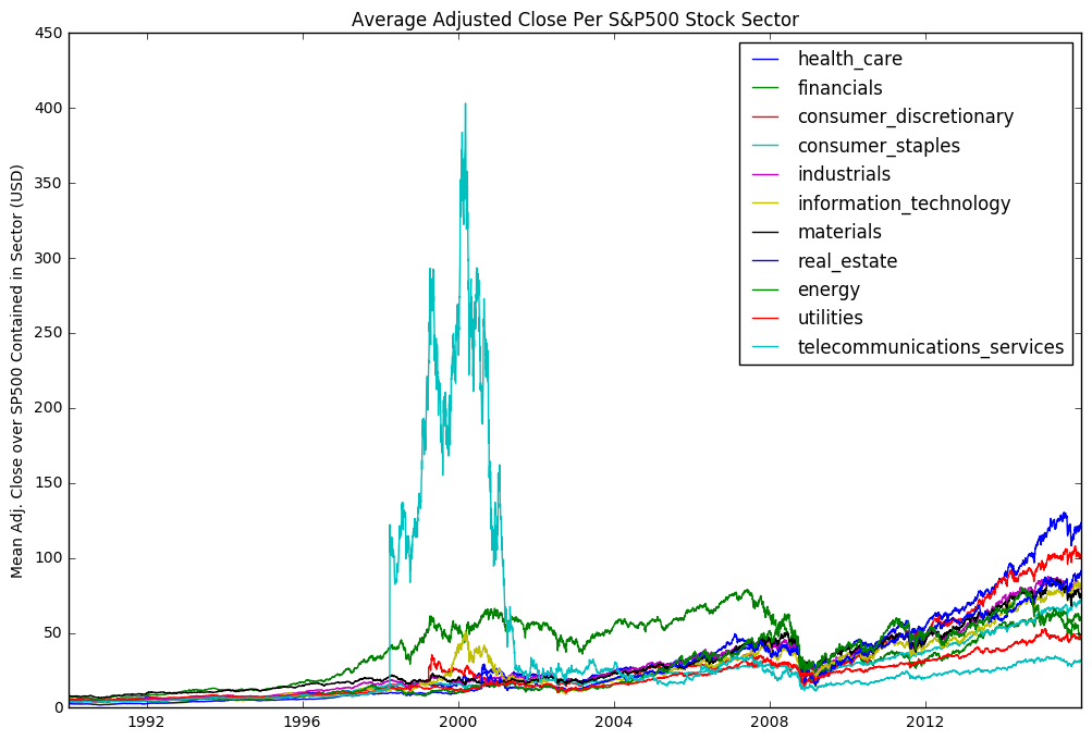
Once we have our data, we can analyse it in any way we want. Below I’ve done some basic plots across all sectors where we can see some historical trends both within sectors and across all sectors
import pandas as pd
import numpy as np
import matplotlib.pyplot as plt
test = pd.DataFrame([np.mean(sector_ohlc[sector]["Adj Close"],axis=1) for sector in list(sector_ohlc.keys())]).T
test.columns = list(sector_ohlc.keys())
plt.figure(figsize = (12,8))
plt.plot(test)
plt.legend(test.columns, loc="best")
plt.ylabel("Mean Adj. Close over SP500 Contained in Sector (USD)")
plt.title("Average Adjusted Close Per S&P500 Stock Sector")
plt.show()
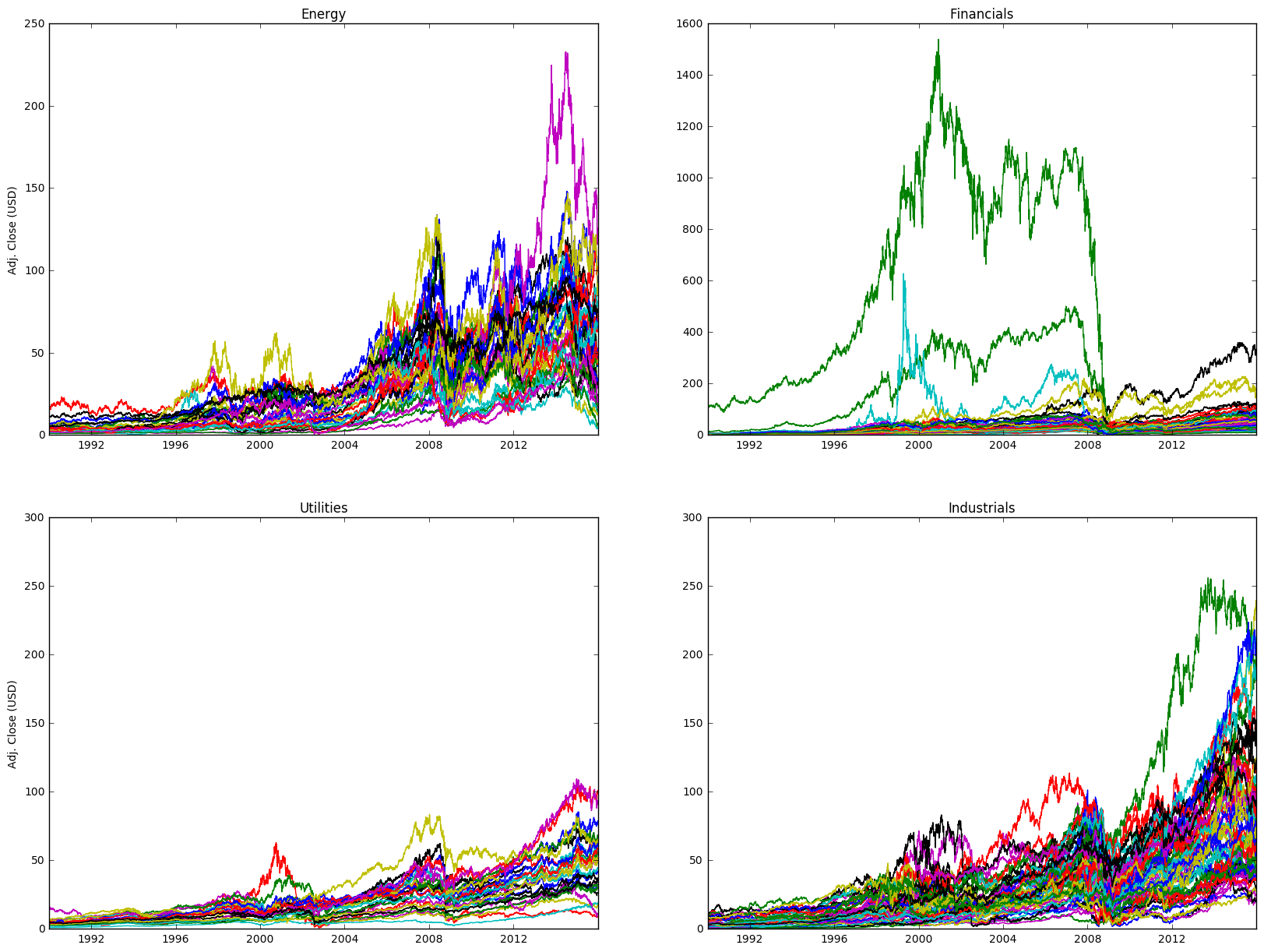
fig = plt.figure(figsize=(20,15))
ax1 = fig.add_subplot(221, title = "Energy", ylabel = "Adj. Close (USD)")
ax2 = fig.add_subplot(222, sharex=ax1, title = "Financials")
ax3 = fig.add_subplot(223, sharex=ax1, title = "Utilities", ylabel = "Adj. Close (USD)")
ax4 = fig.add_subplot(224, sharex=ax1, sharey=ax3, title = "Industrials")
ax1.plot(sector_ohlc["energy"]["Adj Close"])
ax2.plot(sector_ohlc["financials"]["Adj Close"])
ax3.plot(sector_ohlc["utilities"]["Adj Close"])
ax4.plot(sector_ohlc["industrials"]["Adj Close"])
plt.show()
Scraping Fundamental Data - Good Morning
There’s a great package here which allows us to access an API to download a whole bunch of fundamental data. To work, you simply need to download the scripts into a directory and then import them. It also lets us write to our database really easily, and so we can create a store of fundamental securities data.
The Good Morning package also provides a way for us to write to a database, allowing us to keep a nice store of fundamental data. A scraping script is provided which will pull data for the S&P500, and it’s quite easy to substitute in any list of tickers and pull data. If we open up the good_download file we just need to inpute our database details, whatever list of tickers we want to iterate over, and then run the script.
The Good Morning package is fairly easy to follow, so I’ll focus on the subsequent extraction and analysis of data.
Accessing Fundamentals Database
Our data is stored in a SQL database, so we’ll use pymysql to access it.
import pymysql
from sqlalchemy import create_engine
import pandas as pd
import matplotlib.pyplot as plt

# Start connection to mysql database
conn = pymysql.connect(host = 'localhost', user = 'username', password ='password', db = 'mstar', port = 3306)

# Initialise sql engine
engine = create_engine('mysql+pymysql://username:password@localhost:3306/mstar')

# Execute SQL to retrieve from a table
with engine.connect() as conn, conn.begin():
    data = pd.read_sql('select * from morningstar_key_financials_aud;', conn)

with engine.connect() as conn, conn.begin():
    df = pd.read_sql('select * from morningstar_key_profitability;', conn)

df["period"] = pd.to_datetime(df["period"])
data.info()
<class 'pandas.core.frame.DataFrame'>
RangeIndex: 9124 entries, 0 to 9123
Data columns (total 17 columns):
ticker                          9124 non-null object
period                          9124 non-null object
revenue_aud_mil                 4441 non-null float64
gross_margin_percent            2944 non-null float64
operating_income_aud_mil        7182 non-null float64
operating_margin_percent        3487 non-null float64
net_income_aud_mil              7194 non-null float64
earnings_per_share_aud          6207 non-null float64
dividends_aud                   1467 non-null float64
payout_ratio_percent            1206 non-null float64
shares_mil                      7419 non-null float64
book_value_per_share_aud        6117 non-null float64
operating_cash_flow_aud_mil     7141 non-null float64
cap_spending_aud_mil            6111 non-null float64
free_cash_flow_aud_mil          7148 non-null float64
free_cash_flow_per_share_aud    4990 non-null float64
working_capital_aud_mil         6503 non-null float64
dtypes: float64(15), object(2)
memory usage: 1.2+ MB
Plotting/Analysis of Fundamentals
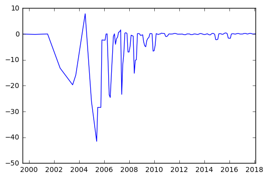
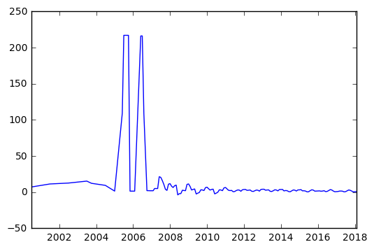
dividends = data.groupby(["period"]).mean()["dividends_aud"]

div_rm = dividends.rolling(min_periods=1, center = True, window = 6).mean().dropna()
plt.plot(div_rm)
plt.xlim([min(div_rm.index), max(div_rm.index)])
plt.show()

eps = data.groupby(["period"]).mean()["earnings_per_share_aud"]

eps_rm = eps.rolling(min_periods=1, center = True, window = 3).mean().dropna()
plt.plot(eps_rm)
plt.xlim([min(eps_rm.index), max(eps_rm.index)])
plt.show()

bv = data.groupby(["period"]).mean()["book_value_per_share_aud"]

bv_rm = bv.rolling(min_periods=1, center = True, window = 3).mean().dropna()
plt.plot(bv_rm)
plt.xlim([min(bv_rm.index), max(bv_rm.index)])
plt.show()
eps = data.groupby(["period"]).mean()
eps.describe()
| revenue_aud_mil | gross_margin_percent | operating_income_aud_mil | operating_margin_percent | net_income_aud_mil | earnings_per_share_aud | dividends_aud | payout_ratio_percent | shares_mil | book_value_per_share_aud | operating_cash_flow_aud_mil | cap_spending_aud_mil | free_cash_flow_aud_mil | free_cash_flow_per_share_aud | working_capital_aud_mil | |
|---|---|---|---|---|---|---|---|---|---|---|---|---|---|---|---|
| count | 120.000000 | 98.000000 | 141.000000 | 113.000000 | 141.000000 | 139.000000 | 91.000000 | 83.000000 | 143.000000 | 131.000000 | 136.000000 | 132.000000 | 136.000000 | 117.000000 | 131.000000 |
| mean | 1183.816251 | 25.882255 | 105.140340 | -58.316214 | 97.141647 | -1.970208 | 0.518721 | 111.158980 | 249.893458 | 6.417518 | 132.222161 | -58.919226 | 80.218256 | -2.782512 | 35.871756 |
| std | 1776.000543 | 33.253144 | 406.449570 | 137.493206 | 244.636578 | 8.194562 | 0.476687 | 86.110656 | 219.201638 | 26.727140 | 568.094339 | 158.001655 | 539.429030 | 15.867349 | 915.190192 |
| min | 0.000000 | -144.700000 | -707.000000 | -943.100000 | -166.500000 | -56.887222 | 0.010000 | 10.000000 | 0.000000 | -10.022851 | -2279.750000 | -1232.000000 | -2433.125000 | -163.756667 | -5813.500000 |
| 25% | NaN | NaN | NaN | NaN | NaN | NaN | NaN | NaN | NaN | NaN | NaN | NaN | NaN | NaN | NaN |
| 50% | NaN | NaN | NaN | NaN | NaN | NaN | NaN | NaN | NaN | NaN | NaN | NaN | NaN | NaN | NaN |
| 75% | NaN | NaN | NaN | NaN | NaN | NaN | NaN | NaN | NaN | NaN | NaN | NaN | NaN | NaN | NaN |
| max | 8366.500000 | 96.800000 | 1904.333333 | 106.800000 | 1147.333333 | 7.866000 | 1.870000 | 714.200000 | 1064.000000 | 217.055556 | 3124.166667 | 0.000000 | 2854.555556 | 14.775000 | 6672.333333 |
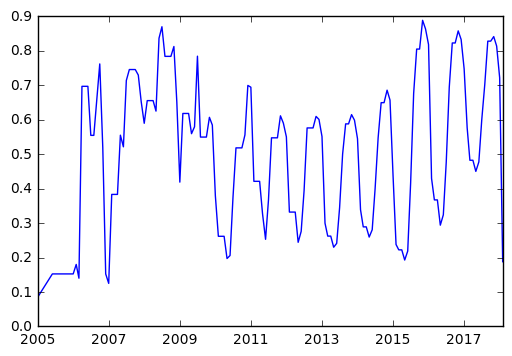
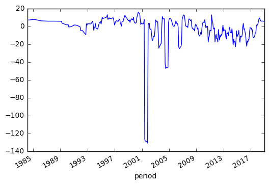
We can see below some potential issues in our data, with some very large drops in 2001, 2005 and 2008. Obviously before using this data for anything meaningful, we’d want to dive in and see what’s driving these issues. It’s possible that there’s a single stock which is significantly off and causing this.
df.head()
mean_profits = df.groupby(["period"]).mean()
mp_rm = mean_profits["return_on_invested_capital_percent"].rolling(min_periods=1, center = True, window = 6).mean().dropna()
mp_rm.plot()
plt.show()
Screening
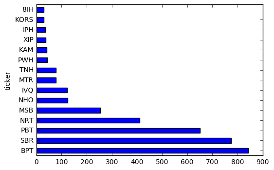
One of the key uses of fundamental data is in screening a list of stocks for certain characteristics. We can pretty easily apply any type of screen we please to our data.
basic_screener = df.groupby(["ticker"])
basic_screener["return_on_assets_percent"].mean().sort_values(ascending = False)[0:15].plot(kind="barh")
plt.show()
period_screener = df[df["period"] > "2014-01-01"]
period_screener = period_screener.groupby(["ticker"])

screen_average = period_screener.mean()
filtered_average = screen_average[(screen_average["return_on_equity_percent"].values > 15) & (screen_average["return_on_equity_percent"].values <= 100)]
filtered_average.sort_values(by = "return_on_equity_percent",ascending = False)[0:15]#.plot(kind="barh")
| tax_rate_percent | net_margin_percent | asset_turnover_average | return_on_assets_percent | financial_leverage_average | return_on_equity_percent | return_on_invested_capital_percent | interest_coverage | |
|---|---|---|---|---|---|---|---|---|
| ticker | ||||||||
| NAH | 7.627500 | 18.120000 | 2.665000 | 47.670000 | 1.945000 | 99.335000 | 99.335000 | NaN |
| BTH | NaN | 16.765000 | 1.550000 | 25.905000 | 2.190000 | 98.465000 | 63.460000 | -0.490000 |
| BA | 18.882500 | 5.427500 | 1.000000 | 5.407500 | 61.667500 | 97.195000 | 33.695000 | 21.962500 |
| IPH | 21.500000 | 29.440000 | 1.133333 | 35.033333 | 1.606667 | 96.136667 | 55.876667 | 46.543333 |
| MAR | 32.645000 | 5.132500 | 1.630000 | 8.655000 | 4.510000 | 88.290000 | 12.670000 | 7.775000 |
| GXY | NaN | NaN | NaN | 26.490000 | 1.420000 | 87.515000 | 70.555000 | 5.945000 |
| OKE | 22.237500 | 3.410000 | 0.590000 | 1.987500 | 60.717500 | 85.675000 | 6.855000 | 2.907500 |
| GILD | 19.362500 | 48.240000 | 0.685000 | 33.457500 | 2.772500 | 85.320000 | 43.790000 | 26.755000 |
| OEC | 34.736667 | 2.070000 | 1.130000 | 1.962500 | 18.947500 | 85.246667 | 49.836667 | 2.310000 |
| SHW | 30.280000 | 9.032500 | 1.897500 | 17.175000 | 4.895000 | 85.242500 | 35.530000 | 17.342500 |
| TWD | 30.310000 | 7.225000 | 4.960000 | 35.965000 | 2.267500 | 81.195000 | 79.892500 | NaN |
| YUM | 26.242500 | 17.160000 | 1.260000 | 18.967500 | 7.125000 | 80.910000 | 23.680000 | NaN |
| IBM | 11.165000 | 14.705000 | 0.720000 | 10.567500 | 7.632500 | 79.102500 | 22.482500 | 29.625000 |
| KAM | 30.665000 | 36.833333 | 0.800000 | 36.947500 | 1.795000 | 78.170000 | NaN | NaN |
| NVO | 20.896667 | 31.953333 | 1.260000 | 40.223333 | 1.990000 | 77.536667 | 73.400000 | 505.383333 |
Binning
Another quick tool I found is binning of our data, we might be interested in a particular subsector of the market and we might want to bin our data into categories. We might, for example, find that a certain sector has a much higher proportion of fundamental ratios being placed into a higher category.
def get_stats(group):
    return {'min': group.min(), 'max': group.max(), 'count': group.count(), 'mean': group.mean()}

bins = [-500, -100, 0, 100, 500]
group_names = ['Very Poor', 'Poor', 'Nil', 'Okay']
data['categories'] = pd.cut(data['earnings_per_share_aud'], bins, labels=group_names)

data['earnings_per_share_aud'].groupby(data['categories']).apply(get_stats).unstack()
| count | max | mean | min | |
|---|---|---|---|---|
| categories | ||||
| Very Poor | 15.0 | -121.31 | -269.578000 | -458.85 |
| Poor | 4178.0 | -0.01 | -0.694816 | -91.93 |
| Nil | 1998.0 | 42.67 | 0.425676 | 0.01 |
| Okay | 2.0 | 414.51 | 327.555000 | 240.60 |
Accessing Pricing Data
We’ve got a database of pricing data, split between daily pricing data and some attribute tables (symbols etc). We’ll write some basic SQL, extract the data and apply some basic transformations/analyses to show how easy it is to run quick analysis across some large sets of data.
import pymysql
from sqlalchemy import create_engine
import pandas as pd
import matplotlib.pyplot as plt
import pandas.io.sql as psql

db_host = 'localhost'
db_user = 'username'
db_pass = 'password'
db_name = 'pricing'

con = pymysql.connect(db_host, db_user, db_pass, db_name)
Reading a Single Ticker
# Select all of the historic Google adjusted close data for symbol MQG

sql = """SELECT *
         FROM symbol AS sym
         INNER JOIN daily_price AS dp
         ON dp.symbol_id = sym.id
         WHERE sym.ticker = 'MQG'
         ORDER BY dp.price_date ASC;"""

engine = create_engine('mysql+pymysql://username:password@localhost:3306/pricing')

# Create a pandas dataframe from the SQL query
with engine.connect() as conn, conn.begin():
    p_data = pd.read_sql(sql, con)
Processing a Single Ticker
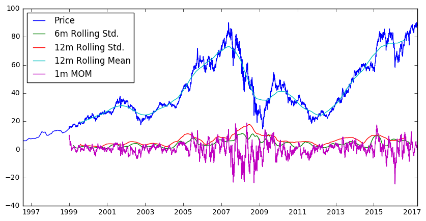
p_data["price_date"] = pd.to_datetime(p_data["price_date"])
df = p_data.groupby(['price_date', 'ticker']).close_price.mean().unstack()
plt.figure(figsize=(10,5))

plt.plot(df)
plt.plot(df.rolling(180, center=True).std())
plt.plot(df.rolling(360, center=True).std())
plt.plot(df.rolling(360, center=True).mean())
plt.plot(df.diff(30))

plt.legend(["Price", "6m Rolling Std.", "12m Rolling Std.", "12m Rolling Mean", "1m MOM"], loc = "best")
plt.yaxis("Adj. Price ($)")
plt.show()
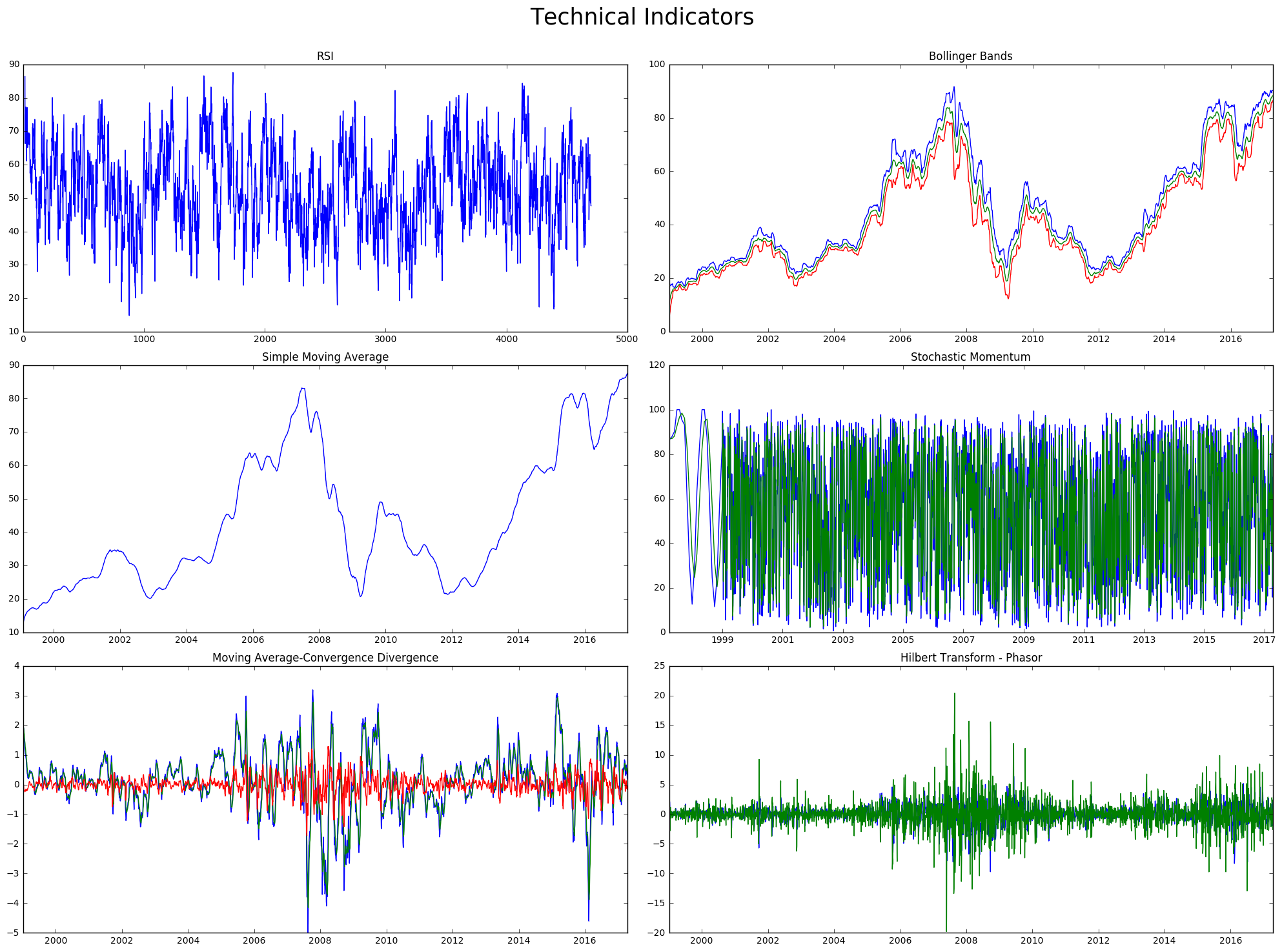
Technical Indicators
We can use the talib libray to get some technical indicators for our chosen ticker.
import talib as ta

inputs = {
    'open': np.array(p_data["open_price"]),
    'high': np.array(p_data["high_price"]),
    'low': np.array(p_data["low_price"]),
    'close': np.array(p_data["close_price"]),
    'volume': np.array(p_data["volume"])
}

fig = plt.figure(figsize = (20,15))
plt.suptitle("Technical Indicators", fontsize = 25)
plt.subplot(321)
plt.plot(ta.RSI(np.array(p_data["close_price"])))
plt.title("RSI")

plt.subplot(322)
upper, middle, lower = ta.BBANDS(np.array(p_data["close_price"]), 30,2,2)
plt.plot(p_data["price_date"],upper)
plt.plot(p_data["price_date"],middle)
plt.plot(p_data["price_date"],lower)
plt.title("Bollinger Bands")


plt.subplot(323)
output = ta.SMA(inputs["close"], 50)
plt.plot(p_data["price_date"],output)
plt.title("Simple Moving Average")

plt.subplot(324)
slowk, slowd = ta.STOCH(inputs["high"], inputs["low"], inputs["close"], 5, 3, 0, 3, 0) # uses high, low, close by default
plt.plot(p_data["price_date"],slowk)
plt.plot(p_data["price_date"],slowd)
plt.title("Stochastic Momentum")

plt.subplot(325)
macd, macdsignal, macdhist = ta.MACD(inputs["close"], fastperiod=12, slowperiod=26, signalperiod=9)
plt.plot(p_data["price_date"],macd)
plt.plot(p_data["price_date"],macdsignal)
plt.plot(p_data["price_date"],macdhist)
plt.title("Moving Average-Convergence Divergence")

plt.subplot(326)
inphase, quadrature = ta.HT_PHASOR(inputs["close"])
plt.plot(p_data["price_date"],inphase)
plt.plot(p_data["price_date"],quadrature)
plt.title("Hilbert Transform - Phasor")

fig.tight_layout()
fig.subplots_adjust(top=0.92)
plt.show()
Reading in All Tickers Post-2015
con = pymysql.connect(db_host, db_user, db_pass, db_name)

sql = """SELECT *
         FROM symbol AS sym
         INNER JOIN daily_price AS dp
         ON dp.symbol_id = sym.id
         where price_date > '2015-01-01';"""

engine = create_engine('mysql+pymysql://username:password@localhost:3306/pricing')

# Create a pandas dataframe from the SQL query
with engine.connect() as conn, conn.begin():
    p_data_full = pd.read_sql(sql, con)
p_data_full.head()
| id | exchange_id | ticker | instrument | name | sector | currency | created_date | last_updated_date | id | ... | symbol_id | price_date | created_date | last_updated_date | open_price | high_price | low_price | close_price | adj_close_price | volume | |
|---|---|---|---|---|---|---|---|---|---|---|---|---|---|---|---|---|---|---|---|---|---|
| 0 | 1 | None | MMM | stock | 3M Company | industrials | USD | 2017-04-16 11:17:25 | 2017-04-16 11:17:25 | 1 | ... | 1 | 2017-04-13 | 2017-04-16 11:18:05 | 2017-04-16 11:18:05 | 189.25 | 189.86 | 188.62 | 188.65 | 188.65 | 1256400 |
| 1 | 1 | None | MMM | stock | 3M Company | industrials | USD | 2017-04-16 11:17:25 | 2017-04-16 11:17:25 | 2 | ... | 1 | 2017-04-12 | 2017-04-16 11:18:05 | 2017-04-16 11:18:05 | 190.31 | 190.49 | 189.40 | 189.70 | 189.70 | 1412600 |
| 2 | 1 | None | MMM | stock | 3M Company | industrials | USD | 2017-04-16 11:17:25 | 2017-04-16 11:17:25 | 3 | ... | 1 | 2017-04-11 | 2017-04-16 11:18:05 | 2017-04-16 11:18:05 | 189.13 | 190.09 | 188.99 | 190.07 | 190.07 | 1454200 |
| 3 | 1 | None | MMM | stock | 3M Company | industrials | USD | 2017-04-16 11:17:25 | 2017-04-16 11:17:25 | 4 | ... | 1 | 2017-04-10 | 2017-04-16 11:18:05 | 2017-04-16 11:18:05 | 190.16 | 190.52 | 189.31 | 189.71 | 189.71 | 1629100 |
| 4 | 1 | None | MMM | stock | 3M Company | industrials | USD | 2017-04-16 11:17:25 | 2017-04-16 11:17:25 | 5 | ... | 1 | 2017-04-07 | 2017-04-16 11:18:05 | 2017-04-16 11:18:05 | 190.03 | 190.56 | 189.52 | 189.99 | 189.99 | 1012300 |
5 rows × 21 columns
Screening
Typically when reading in all of our symbols, we care more about identifying some overarching information from this dataset i.e. filtering this larger dataset to a smaller subset which we can investigate in more detail.
A filter can be anything you deem relevant to choosing a stock of interest, sectors, currency, time, change, etc.
symlist = pd.DataFrame(np.unique(p_data_full["ticker"]), columns=["ticker"])

def filter_combined(prices):
    mean_12m = prices["close_price"].rolling(360, center=True).mean().mean()
    mean_1m = prices["close_price"].rolling(30, center=True).mean().mean()

    std_12m = prices["close_price"].rolling(360, center=True).std().mean()
    std_1m = prices["close_price"].rolling(30, center=True).std().mean()

    vol_12m = prices["volume"].pct_change(periods=12).mean()
    vol_1m = prices["volume"].pct_change(periods=1).mean()


    return mean_1m / mean_12m, std_1m / std_12m, vol_1m / vol_12m


vals = [filter_combined(p_data_full[p_data_full["ticker"] == sym]) for sym in symlist["ticker"]]
vals = pd.DataFrame(vals)
symlist[["mean_filter", "std_dev_filter", "vol_filter"]] = vals
symlist.sort_values(by=["std_dev_filter"], ascending = False)[0:15]
| ticker | mean_filter | std_dev_filter | vol_filter | |
|---|---|---|---|---|
| 223 | ESS | 1.001476 | 0.627439 | 0.481566 |
| 296 | HGG | 1.011987 | 0.592418 | NaN |
| 146 | CNC | 1.033845 | 0.579133 | 0.379061 |
| 469 | OSH | 1.014487 | 0.573757 | NaN |
| 545 | SFR | 0.992697 | 0.573522 | NaN |
| 68 | AVB | 0.994137 | 0.569020 | 0.637264 |
| 45 | AMGN | 1.006408 | 0.564985 | 0.449691 |
| 654 | WES | 1.011016 | 0.559084 | NaN |
| 311 | HUM | 1.012941 | 0.550026 | 0.404243 |
| 273 | GOZ | 0.998420 | 0.549429 | NaN |
| 614 | TTS | 1.007085 | 0.545860 | NaN |
| 622 | UDR | 0.990442 | 0.533801 | 0.392167 |
| 9 | ABP | 0.993232 | 0.530184 | NaN |
| 649 | WBA | 1.003274 | 0.528790 | 0.531408 |
| 173 | CWN | 1.011845 | 0.525692 | NaN |
Naturally there’s an issue with some of our data, in that our GICS sector codes vary in how they’ve been read into our database. We can apply a fairly easy fix to this.
np.unique(p_data_full["sector"])

def replace_all_keys(s, dict):
    for i, j in dict.items():
        s = s.replace(i, j)
    return s

replacement_key = {"consumer_discretionary": "Consumer Discretionary",
                  "health_care":"Health Care",
                  "real_estate":"Real Estate",
                  "telecommunication_services":"Telecommunication Services",
                  "information_technology":"Information Technology",
                  "consumer_staples":"Consumer Staples",
                  "utilities":"Utilities",
                  "financials":"Financials",
                  "energy":"Energy",
                  "materials":"Materials",
                  "industrials":"Industrials"}

p_data_full = p_data_full.apply(lambda x: replace_all_keys(x, replacement_key))
p_data_sector = p_data_full.groupby(["sector", "price_date"])

plt.figure(figsize = (15,10))
vals = p_data_sector["volume"].mean().unstack(level=0)
vals.ewm(span=20).mean().plot()
plt.legend(bbox_to_anchor=(1.7,1))
plt.ylabel("Volume")
plt.show()
<matplotlib.figure.Figure at 0xbd44aecf28>
Areas to Fix/Explore
Fundamentals
- More advanced binning of data analysis, as opposed to just the single factor.
Pricing
- Incorporate technical indicators into database, to create filters/signals for stock identification (i.e. if current price is > 200 day SMA etc)
- Look at gaps in pricing data.