Textual Analysis of The Office (US) Transcripts
Here we’ll do a quick review of everybody’s favourite television show, The Office (US version of course)! We’ll pull out some basic statistics, run some bag-of-words analysis to look at how often characters are interacting. We’ll finish up with some VADER sentiment analysis to see how each Season is tracking!
Data graciously obtained from here
import pandas as pd
import numpy as np
import matplotlib.pyplot as plt
from matplotlib import cm
import seaborn as sns

import re
from nltk.corpus import stopwords
from nltk.sentiment import SentimentAnalyzer
from nltk.sentiment.vader import SentimentIntensityAnalyzer
from nltk import tokenize

from sklearn.feature_extraction.text import CountVectorizer
Data Import & Basic Preprocessing
Here we do a bit of cleaning to remove any unwanted punctuation, convert everything to lower case and remove any stopwords using NLTK.
df = pd.read_excel("D:\\Downloads\\the-office-lines.xlsx")
df['speaker'] = [w.lower() for w in df['speaker']]
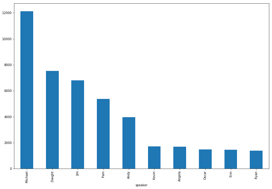
df.groupby(['speaker'])['id'].count().sort_values(ascending=False)[0:10].plot(kind='bar', figsize=(15,10))
plt.show()
def clean_words(raw_string, clean_characters=False, characters=None):
    raw_string = str(raw_string)
    cleaned = [w for w in re.sub("[^a-zA-Z]", " ", raw_string).lower().split()]
    stops = set(stopwords.words("english"))
    cleaned = [w for w in cleaned if not w in stops]

    # if we want to only look at characters saying certain words (i.e. other characters)
    if clean_characters:
        cleaned = [w for w in cleaned if w in characters]
    return (" ".join(cleaned))
def gen_cleaned_script(df, clean_characters=False, characters=None):

    cleaned_script = []

    for i in range(0, df.shape[0]):
        if((i+1) % 5000 == 0):
            print("Review %d of %d\n" % (i+1, df.shape[0]))
        #cleaned_script.append(clean_words(df['line_text'][i]))
        cleaned_script.append(clean_words(df['line_text'][i], clean_characters, main_characters_lower))

    return cleaned_script
cleaned_script_all = gen_cleaned_script(df)
cleaned_script_characters = gen_cleaned_script(df, True, main_characters_lower)
Review 5000 of 59909

Review 10000 of 59909

Review 15000 of 59909

Review 20000 of 59909

Review 25000 of 59909

Review 30000 of 59909

Review 35000 of 59909

Review 40000 of 59909

Review 45000 of 59909

Review 50000 of 59909

Review 55000 of 59909

Review 5000 of 59909

Review 10000 of 59909

Review 15000 of 59909

Review 20000 of 59909

Review 25000 of 59909

Review 30000 of 59909

Review 35000 of 59909

Review 40000 of 59909

Review 45000 of 59909

Review 50000 of 59909

Review 55000 of 59909
Count Analysis
The first basic analysis we can do is to look at the most common words used across the entire script. Not that interesting, but we can apply to the entire script as well as on a character by character level if we so choose (or even a specific subset of words).
When combined with clean_words() above, we can effectively run count analyses on any set of words we wish (i.e. all words in the script, character names, location references, etc etc.). We’ll first show how to run this across ALL data
def get_word_counts(text):

    vectorizer = CountVectorizer(analyzer="word", tokenizer=None, preprocessor=None, stop_words=None, max_features=5000)

    train = vectorizer.fit_transform(text)
    train = train.toarray()
    vocab = vectorizer.get_feature_names()

    dist = np.sum(train, axis=0)

    combined_vocab = pd.DataFrame(vocab)
    combined_vocab = combined_vocab.merge(pd.DataFrame(dist), left_index=True, right_index=True)
    combined_vocab.columns = ['Word', 'Count']
    combined_vocab.sort_values(by='Count', ascending=False)
    combined_vocab.set_index('Word', inplace=True)

    return combined_vocab
all_vals = get_word_counts(cleaned_script_all)
all_vals.sort_values(by='Count', ascending=False)[0:10]
| Count | |
|---|---|
| Word | |
| know | 4434 |
| oh | 4323 |
| like | 3369 |
| yeah | 3227 |
| okay | 2975 |
| michael | 2861 |
| right | 2700 |
| get | 2613 |
| well | 2508 |
| hey | 2421 |
michael = np.array(cleaned_script_all)[[(df.loc[df.speaker == 'michael'].index.values)]]
michael_counts = get_word_counts(michael)
michael_counts.sort_values(by='Count', ascending=False)[0:20]
| Count | |
|---|---|
| Word | |
| know | 1369 |
| oh | 1039 |
| okay | 984 |
| like | 882 |
| well | 821 |
| right | 818 |
| go | 749 |
| going | 736 |
| good | 728 |
| get | 662 |
| yeah | 631 |
| think | 591 |
| dwight | 588 |
| want | 571 |
| would | 566 |
| yes | 563 |
| hey | 554 |
| one | 524 |
| pam | 511 |
| ok | 484 |
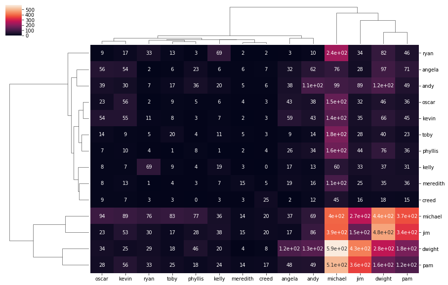
Now that we’ve run the analysis for one character, we can run this analysis across all characters to see who is saying each others names the most! Not unexpectedly, we see the four main characters (Michael, Jim, Dwight and Pam) dominating the charts. With Michael in particular having a large amount of intereaction across pretty much every other characters name.
vals = pd.DataFrame(index=main_characters_lower, columns=main_characters_lower)

for i in main_characters_lower:
    tmp = np.array(cleaned_script_characters)[[(df.loc[df.speaker == i].index.values)]]
    vals[i] = get_word_counts(tmp)

vals.fillna(0, inplace=True)
sns.clustermap(vals, annot=True, figsize=(15,10))
plt.show()
Sentiment Analysis using VADER
Perhaps more interesting is to look at how positive/negative/neutral each of the characters lines are, how they’ve varied over time and how they correlate with each other. Note that the correlation is not necessarily due to the characters interacting with each other, but just there general mood within each season. I.e. if we see a positive correlation, it means that within that season both of those characters generall had, on average, positive sentiment in their lines.
sentiment = []

for i in range(0, df.shape[0]):
    if((i+1) % 5000 == 0):
        print("Review %d of %d\n" % (i+1, df.shape[0]))
    sentiment.append(sid.polarity_scores(str(cleaned_script[i])))

sentiment = pd.DataFrame(sentiment)
df_sentiment = df.merge(sentiment, left_index=True, right_index=True)
Review 5000 of 59909

Review 10000 of 59909

Review 15000 of 59909

Review 20000 of 59909

Review 25000 of 59909

Review 30000 of 59909

Review 35000 of 59909

Review 40000 of 59909

Review 45000 of 59909

Review 50000 of 59909

Review 55000 of 59909
main_characters = ['Michael', 'Jim', 'Dwight', 'Pam', 'Angela', 'Toby', 'Phyllis', 'Andy', 'Oscar', 'Kevin',
                  'Meredith', 'Creed', 'Kelly', 'Ryan']
main_characters_lower = [w.lower() for w in main_characters]
out = df_sentiment.loc[df_sentiment.speaker.isin(main_characters)].groupby(['season', 'speaker'])['compound'].sum().unstack()
out.fillna(0, inplace=True)
corrmat = np.corrcoef(out.T)
corrmat = pd.DataFrame(corrmat, columns=out.columns, index=out.columns)
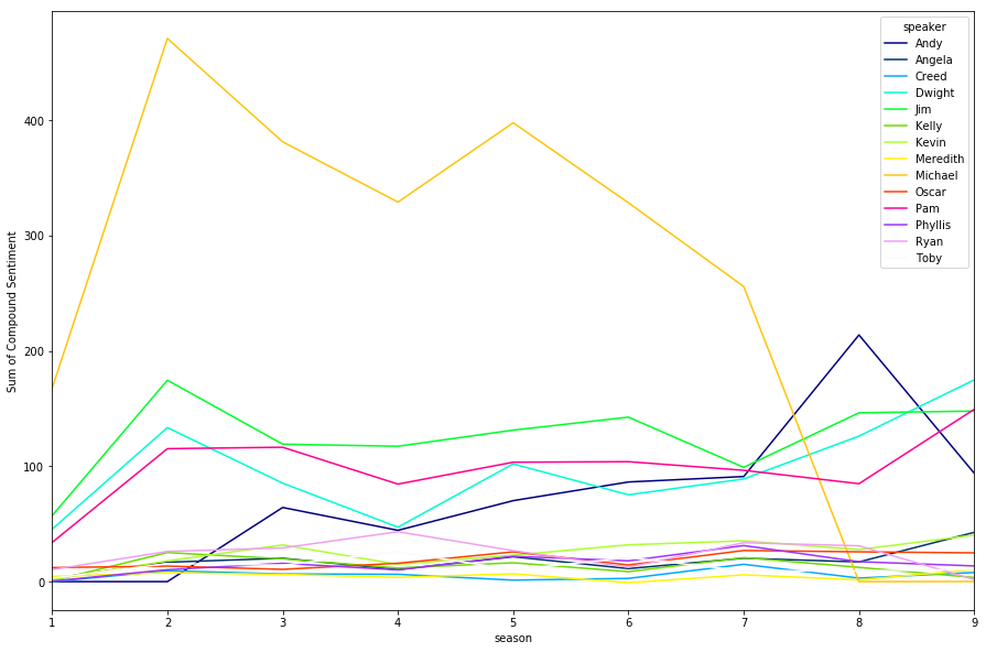
Having done our primitive VADER analysis across each character and season, we can start to look at the trends. My favourite one popping up is the change in Michael from Season 1 to Season 2. It’s a well known fact that there was a creative change in the direction of Michael’s character from a terrible, overbearing boss (more similar to the Ricky Gervais version), to a much more likeable goofball. We see this reflected in the stark transition in the compound sentiment of his character.
It should be noted that because we’re taking the aggregate across each character, it will be influenced by the amount of lines the character has. We could use the mean but the results weren’t substantially different…
out.plot(figsize=(15,10), cmap = cm.get_cmap('gist_ncar'))
plt.ylabel('Sum of Compound Sentiment')
plt.show()
plt.figure(figsize=(15,10))
sns.clustermap(corrmat)
plt.show()
<matplotlib.figure.Figure at 0x1b01e78ab00>
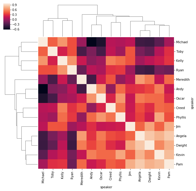
Now that we’ve seen the polarising impact of Michael, we can look at the “aggregate” sum of correlation across each character. This should effectively tell us who shares the most consistent positive/negative sentiment across a season with all of the other characters. Not unsurprisingly we see Pam, Kevin and Phyllis topping these charts, the characters who aren’t really conflict starters. Interestingly we also see Angela up there…not sure how to explain that one just yet.
Right down the bottom we see Michael, Toby, Ryan and Andy who were all characters up for some conflict… typically with each other.
corrmat.sum(axis=1).sort_values().plot(kind='bar')
plt.show()