CryptoCurrency Data Analysis & Primitive Trading
Dataset: https://www.kaggle.com/natehenderson/top-100-cryptocurrency-historical-data
This post is purely for fun/demonstrative purposes… nobody should actually take any investment advice or purchase cryptocurrency based on primitive trading strategies/analysis.
import pandas as pd
import numpy as np
import matplotlib.pyplot as plt
import glob
import datetime as dt

import seaborn as sns

import warnings
warnings.filterwarnings('ignore')
path =r'D:\Downloads\Coding\Datasets\CryptoCurrencyHistoricalData' # use your path
allFiles = glob.glob(path + "/*.csv")
frame = pd.DataFrame()
list_ = []
for file_ in allFiles:
    df = pd.read_csv(file_, delimiter=";")
    list_.append(df)
frame = pd.concat(list_)
close_df = pd.merge(list_[0].iloc[:,[0,4]], list_[1].iloc[:,[0,4]], how = "outer", on="Date")

for i in range(2,len(list_)):
    close_df = pd.merge(close_df, list_[i].iloc[:,[0,4]], how = "outer", on="Date")

names = []
for i in range(0, len(allFiles)):
    names.append(allFiles[i].split(path+"\\")[1].split(".csv")[0])
names.insert(0, "Date")
close_df.columns = names
close_df = close_df.fillna(0)

close_df.Date[96] = '18/08/2017'
close_df.Date[672] = '18/08/2016'
close_df.Date[827] = '18/08/2015'
close_df.Date[1192] = '18/08/2014'
close_df.Date[1557] = '18/08/2013'

close_df.set_index("Date", inplace=True)
close_df.index = pd.to_datetime(close_df.index, format="%d/%m/%Y")
close_df.sort_index(ascending=True, inplace=True)
mcap_df = pd.merge(list_[0].iloc[:,[0,6]], list_[1].iloc[:,[0,6]], how = "outer", on="Date")

for i in range(2,len(list_)):
    mcap_df = pd.merge(mcap_df, list_[i].iloc[:,[0,6]], how = "outer", on="Date")

mcap_df.columns = names

mcap_df.Date[96] = '18/08/2017'
mcap_df.Date[672] = '18/08/2016'
mcap_df.Date[827] = '18/08/2015'
mcap_df.Date[1192] = '18/08/2014'
mcap_df.Date[1557] = '18/08/2013'

mcap_df.set_index("Date", inplace=True)
mcap_df.index = pd.to_datetime(mcap_df.index)
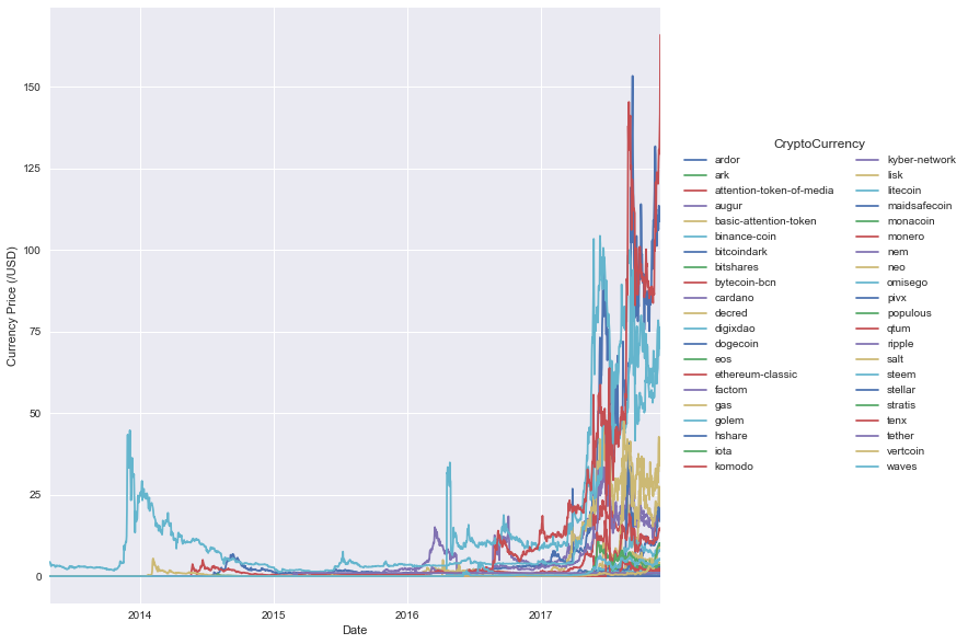
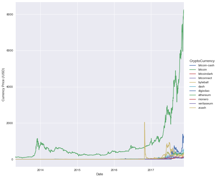
Not unexpectedly, the price profiles of most cryptocurrencies are quite similar…virtually nothing for a while and then explosive growth.
close_df.loc[:,np.max(close_df, axis=0) < 200].plot(figsize=(10,10))
plt.legend(loc="center right", bbox_to_anchor=[1.5, 0.5],
           ncol=2,title="CryptoCurrency")
plt.ylabel("Currency Price (/USD)")
plt.show()
close_df.loc[:,np.max(close_df, axis=0) > 100].plot(figsize=(10,10))
plt.legend(loc="center right", bbox_to_anchor=[1.2, 0.5],
           ncol=1,title="CryptoCurrency")
plt.ylabel("Currency Price (/USD)")
plt.show()
temp_df = pd.concat([close_df['bitcoin'], close_df.loc[:, close_df.columns != 'bitcoin'].shift(1)])
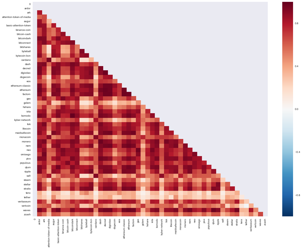
Also not unexpected, we observe some very strong correlation across a large cross-section of the cryptocurrency markets.
corr = temp_df.corr()

mask = np.zeros_like(corr, dtype=np.bool)
mask[np.triu_indices_from(mask)] = True

fig, ax = plt.subplots(figsize=(20,15))
cmap = sns.diverging_palette(220, 10, as_cmap=True)

sns.heatmap(corr, mask=mask)
plt.show()
Basic Trading Strategy
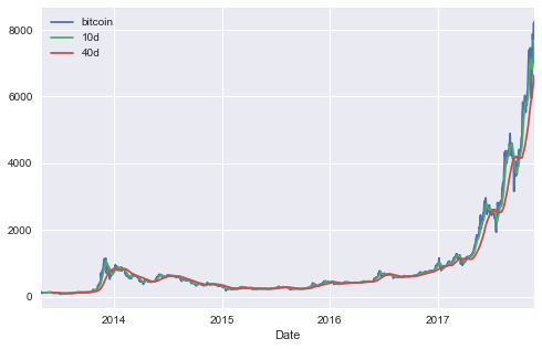
Here we implement a pretty basic trading strategy, where we look at the difference in BTC prices over a certain time-horizon and either buy/sell depending on the direction.
The basic premise is:
- Calculate 10d and 40d average BTC price.
- Choose some target delta between Price_Diff = Price(10d) - Price(40d), and whenever Price_Diff > delta we buy, and when the delta closes we sell.
btc = pd.DataFrame(close_df['bitcoin'], index=close_df.index)
btc.columns = ["bitcoin"]
btc['10d'] = np.round(btc["bitcoin"].rolling(window=10).mean(),2)
btc['40d'] = np.round(btc["bitcoin"].rolling(window=40).mean(),2)
btc[['bitcoin','10d','40d']].plot(grid=True,figsize=(8,5))
plt.show()
We compare our strategy against a simple buy and hold approach. Naturally given the volatility in bitcoin and the astronomical growth, we’d expect that the buy and hold would be incredibly difficult to beat… especially if we started to take into account transaction costs (and potential FX issues if purchasing via a non-USD currency).
Given the huge shift in prices of BTC, we also would prefer to have a dynamically adjusting delta… as using a constant one over even a 6-12 month period will likely result in poor outcomes.
btc = btc[btc.index > pd.datetime(2017,1,1)]
btc['10-40'] = btc['10d'] - btc['40d']
X = 50
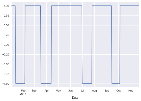
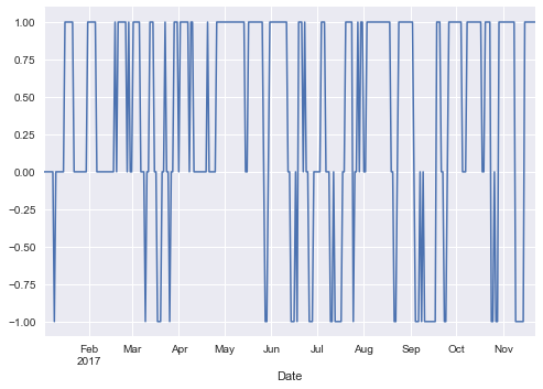
btc['Stance'] = np.where(btc['10-40'] > X, 1, 0)
btc['Stance'] = np.where(btc['10-40'] < X, -1, btc['Stance'])
btc['Stance'].value_counts()
btc['Stance'].plot(lw=1.5,ylim=[-1.1,1.1])
plt.show()
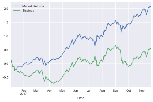
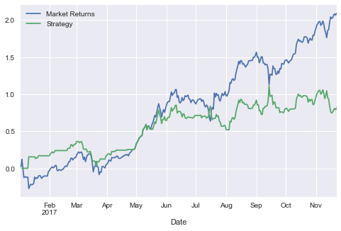
btc['Market Returns'] = np.log(np.float64(btc['bitcoin'] / btc['bitcoin'].shift(1)))
btc['Strategy'] = btc['Market Returns'] * btc['Stance'].shift(1)
btc[['Market Returns','Strategy']].cumsum().plot(grid=True,figsize=(8,5))
plt.show()
Optimisation
As above, we see that our strategy substantially underperforms the simple buy and hold strategy. Now for fun, we can generalise our approach and do some basic optimisation/variable mining.
def annualised_sharpe(returns, N=252):
    return np.sqrt(N) * (returns[~np.isnan(returns)].mean() / returns[~np.isnan(returns)].std())

def bitcoin_sim(btc, shift_time, price_tol, forecast_length):
    btc['diff'] = btc["bitcoin"] - btc["bitcoin"].shift(shift_time)

    btc['Stance'] = np.where(btc['diff'] < -3*price_tol, -1, 0)
    btc['Stance'] = np.where(btc['diff'] > price_tol, 1, btc['Stance'])
   # btc['Stance'].value_counts()

    #btc['Stance'].plot(lw=1.5,ylim=[-1.1,1.1])
    #plt.show()

    btc['Market Returns'] = np.log(np.float64(btc['bitcoin'] / btc['bitcoin'].shift(1)))
    btc['Strategy'] = btc['Market Returns'] * btc['Stance'].shift(forecast_length)

    #btc[['Market Returns','Strategy']].cumsum().plot(grid=True,figsize=(8,5))


    return (btc['Strategy'].cumsum().tail(1), annualised_sharpe(btc['Strategy']))
bitcoin_sim(btc, 1, 1, 1)
(Date
 2017-11-22    0.220979
 Name: Strategy, dtype: float64, 0.24081979662549807)
shift_time = np.linspace(1, 200, 10, dtype=int)
price_tol = np.linspace(-200, 300, 10, dtype=int)
#forecast_length = np.linspace(1, 30, 5, dtype=int)

results_pnl = np.zeros((len(shift_time), len(price_tol)))
results_sharpe = np.zeros((len(shift_time), len(price_tol)))

market_returns = btc['Market Returns'].cumsum().tail(1)
market_sharpe = annualised_sharpe(btc['Market Returns'])


for i, shift_t in enumerate(shift_time):
    for j, price_t in enumerate(price_tol):
        pandl, risk = bitcoin_sim(btc, shift_t, price_t, 1)
        results_pnl[i, j] = pandl - market_returns
        results_sharpe[i, j] = risk - market_sharpe
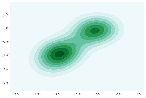
max(results_pnl.flatten())
0.16149115817834314
sns.kdeplot(pd.DataFrame(results_pnl), shade=True)
plt.show()
sns.kdeplot(pd.DataFrame(results_sharpe), shade=True)
plt.show()
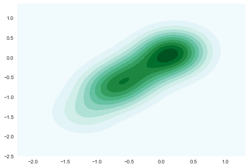
We can take the results out of the above… and look at what the returns profile looks now. We see that our strategy does quite well early on but has substantially lagged the market. Nonetheless, we have a decent framework for investigating very primitive and basic trading strategies.
price_diff_time = 5
price_tol = 50
forecast_horizon = 2

btc['diff'] = btc["bitcoin"] - btc["bitcoin"].shift(price_diff_time)

btc['Stance'] = np.where(btc['diff'] < -3*price_tol, -1, 0)
btc['Stance'] = np.where(btc['diff'] > price_tol, 1, btc['Stance'])
btc['Stance'].value_counts()

btc['Stance'].plot(lw=1.5,ylim=[-1.1,1.1])
plt.show()

btc['Market Returns'] = np.log(np.float64(btc['bitcoin'] / btc['bitcoin'].shift(1)))
btc['Strategy'] = btc['Market Returns'] * btc['Stance'].shift(forecast_horizon)

btc[['Market Returns','Strategy']].cumsum().plot(grid=True,figsize=(8,5))

plt.show()
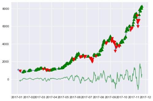
A key feature of a trading strategy that needs to be considered is both turnover and the flowon effect into transaction costs. As expected, because we’re using a small delta we our executing A LOT of buy/sell orders… and naturally we would expect our underperformance to be even worse.
So in conclusion… most people would have likely been better off just buying and holding BTC as opposed to trying to trade based off of any form of technical analysis.
plt.plot(btc.index, btc['bitcoin'], label="Close Price")
plt.plot(btc.ix[btc.Stance == 1]['bitcoin'].index, btc.ix[btc.Stance == 1]['bitcoin'], '^', markersize=10, color='g')
plt.plot(btc.ix[btc.Stance == -1]['bitcoin'].index, btc.ix[btc.Stance == -1]['bitcoin'], 'v', markersize=10, color='r')
plt.plot(btc.index, btc["diff"], label="pricediff")
plt.show()
Extra data to explore
from ggplot import *
df = pd.read_csv(r"D:\Downloads\crypto-markets.csv")
df.date = pd.to_datetime(df.date)
df.head()
| slug | symbol | name | date | ranknow | open | high | low | close | volume | market | close_ratio | spread | |
|---|---|---|---|---|---|---|---|---|---|---|---|---|---|
| 0 | bitcoin | BTC | Bitcoin | 2013-04-28 | 1 | 135.30 | 135.98 | 132.10 | 134.21 | 0 | 1500520000 | 0.5438 | 3.88 |
| 1 | bitcoin | BTC | Bitcoin | 2013-04-29 | 1 | 134.44 | 147.49 | 134.00 | 144.54 | 0 | 1491160000 | 0.7813 | 13.49 |
| 2 | bitcoin | BTC | Bitcoin | 2013-04-30 | 1 | 144.00 | 146.93 | 134.05 | 139.00 | 0 | 1597780000 | 0.3843 | 12.88 |
| 3 | bitcoin | BTC | Bitcoin | 2013-05-01 | 1 | 139.00 | 139.89 | 107.72 | 116.99 | 0 | 1542820000 | 0.2882 | 32.17 |
| 4 | bitcoin | BTC | Bitcoin | 2013-05-02 | 1 | 116.38 | 125.60 | 92.28 | 105.21 | 0 | 1292190000 | 0.3881 | 33.32 |
ggplot(aes(x='date', y='close', color='name'), data=df[df.ranknow <= 10]) + geom_line()
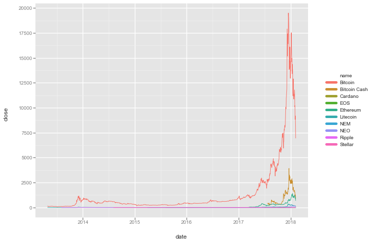
<ggplot: (166606426937)>
* Shifted correlation i.e. what happens to price of other currencies in days after bitocin has large increases