Can We Predict Tomorrow’s Average Rainfall in Australia?

We’ll pull apart the dataset, do the usual EDA, followed up with some time-series decomposition, feature extraction and basic deep learning for forecasting.

Data Source here

import pandas as pd
import numpy as np
import matplotlib.pyplot as plt
import seaborn as sns

Exploration

We can see that the dataset is already setup quite nicely. The initial goal is to predict ‘RainTomorrow’, where the variable has already been setup correctly for analysis. We’ve got all of the typical components: temperature, wind direction, wind speed, humidity and pressure. My initial suspicions are that the 3pm pressure and 3pm humidity components, as well as location, will be the key drivers of whether it will rain tomorrow.

df = pd.read_csv(r"D:\Downloads\weatherAUS.csv\weatherAUS.csv")

df.info()

<class 'pandas.core.frame.DataFrame'>
RangeIndex: 145460 entries, 0 to 145459
Data columns (total 24 columns):
Date             145460 non-null object
Location         145460 non-null object
MinTemp          143975 non-null float64
MaxTemp          144199 non-null float64
Rainfall         142199 non-null float64
Evaporation      82670 non-null float64
Sunshine         75625 non-null float64
WindGustDir      135134 non-null object
WindGustSpeed    135197 non-null float64
WindDir9am       134894 non-null object
WindDir3pm       141232 non-null object
WindSpeed9am     143693 non-null float64
WindSpeed3pm     142398 non-null float64
Humidity9am      142806 non-null float64
Humidity3pm      140953 non-null float64
Pressure9am      130395 non-null float64
Pressure3pm      130432 non-null float64
Cloud9am         89572 non-null float64
Cloud3pm         86102 non-null float64
Temp9am          143693 non-null float64
Temp3pm          141851 non-null float64
RainToday        142199 non-null object
RISK_MM          142193 non-null float64
RainTomorrow     142193 non-null object
dtypes: float64(17), object(7)
memory usage: 26.6+ MB

df.head()

	Date	Location	MinTemp	MaxTemp	Rainfall	Evaporation	Sunshine	WindGustDir	WindGustSpeed	WindDir9am	...	Humidity3pm	Pressure9am	Pressure3pm	Cloud9am	Cloud3pm	Temp9am	Temp3pm	RainToday	RISK_MM	RainTomorrow
0	2008-12-01	Albury	13.4	22.9	0.6	NaN	NaN	W	44.0	W	...	22.0	1007.7	1007.1	8.0	NaN	16.9	21.8	No	0.0	No
1	2008-12-02	Albury	7.4	25.1	0.0	NaN	NaN	WNW	44.0	NNW	...	25.0	1010.6	1007.8	NaN	NaN	17.2	24.3	No	0.0	No
2	2008-12-03	Albury	12.9	25.7	0.0	NaN	NaN	WSW	46.0	W	...	30.0	1007.6	1008.7	NaN	2.0	21.0	23.2	No	0.0	No
3	2008-12-04	Albury	9.2	28.0	0.0	NaN	NaN	NE	24.0	SE	...	16.0	1017.6	1012.8	NaN	NaN	18.1	26.5	No	1.0	No
4	2008-12-05	Albury	17.5	32.3	1.0	NaN	NaN	W	41.0	ENE	...	33.0	1010.8	1006.0	7.0	8.0	17.8	29.7	No	0.2	No

5 rows × 24 columns

df['Date'] = pd.to_datetime(df['Date'])
df['Year-Mon'] = [x.strftime("%Y-%m") for x in df['Date']]

Average Rainfall

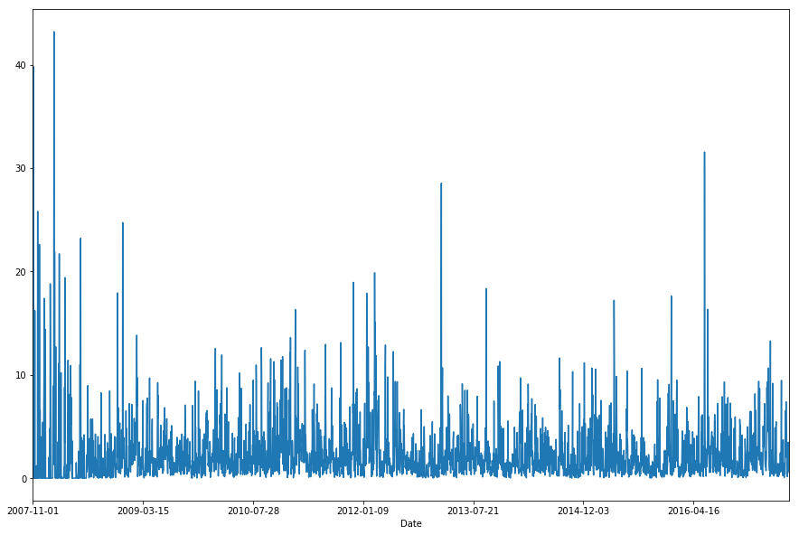
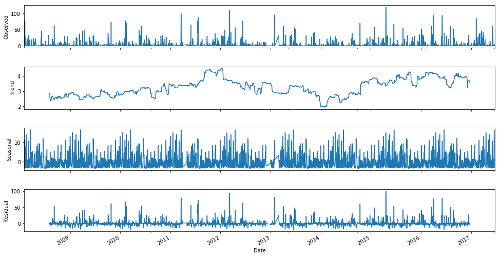
If we look at the daily average rainfall, we can see that it’s pretty noisy (as expected), and quite difficult to see any obvious trends. This is not unexpected as we’ve averaged across the entire location universe, and so we end up with a process that looks quite stationary.

df.groupby(['Date'])['Rainfall'].mean().plot(figsize=(15,10))
plt.show()

png

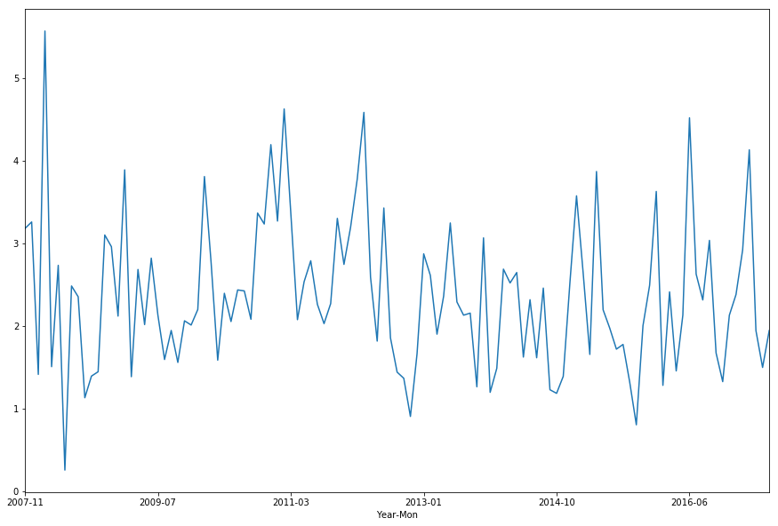
df.groupby(['Year-Mon'])['Rainfall'].mean().plot(figsize=(15,10))
plt.show()

png

Location Analysis

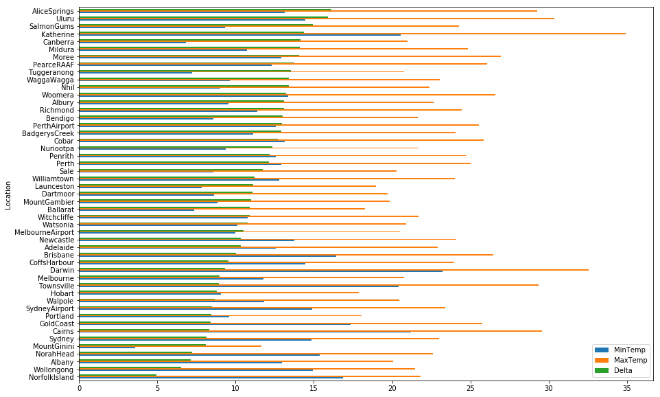
Our dataset isn’t huge, and only has a selection of . If we look at the average min/max temperatures and then take the largest spread, we see that the desert locations have the largest spread, whilst coastal regions seem to be a bit more stable.

temp_avg = df.groupby(['Location']).mean()[['MinTemp', 'MaxTemp']]
temp_avg['Delta'] = temp_avg['MaxTemp'] - temp_avg['MinTemp']
temp_avg.sort_values(by='Delta', ascending=True).plot(kind='barh', figsize=(15,10))
plt.show()

png

Correlations

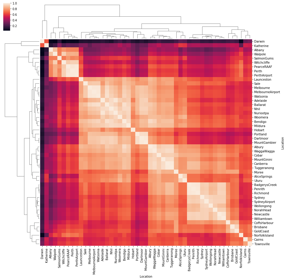
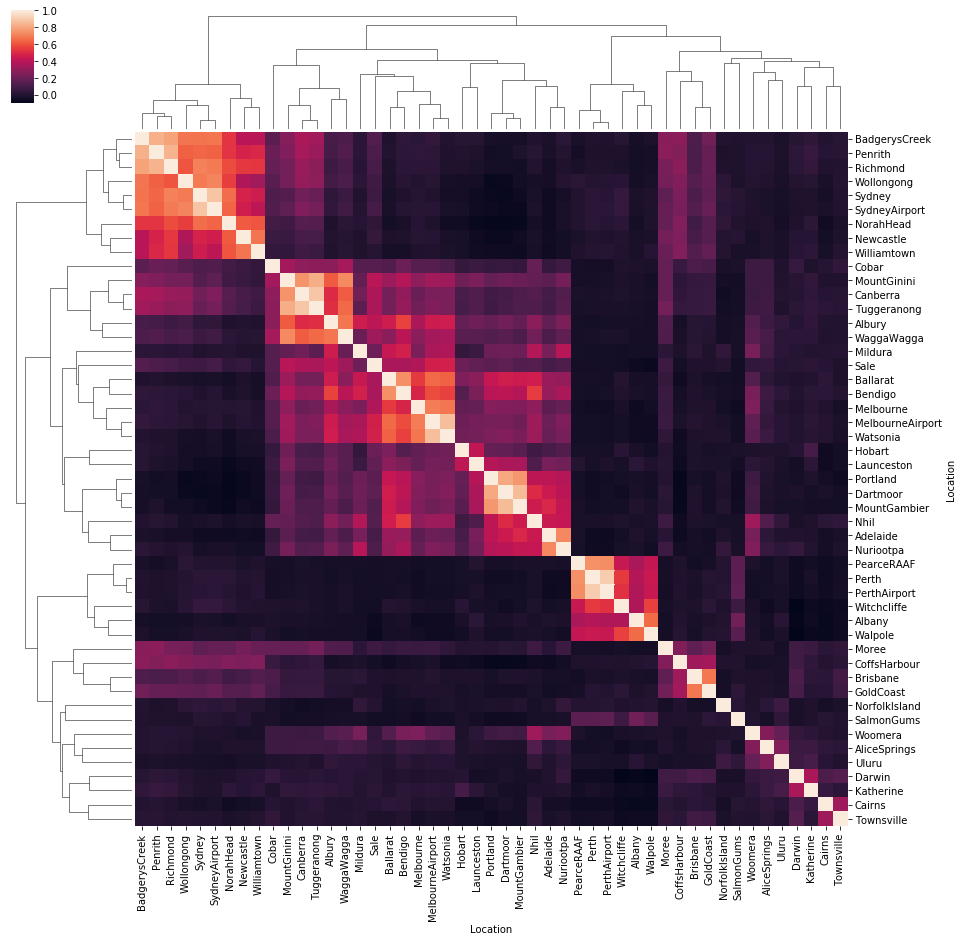
Let’s see if we can pull out some correlations between locations based on temperature and rainfall. We do get ~4-5 clusters of locations with similar rainfall patterns: Sydney region (Sydney, Penrith, Richmond, etc.), Perth, Central Australia and Southern Australia (Melbourne, Tasmania).

temp_by_loc = df.groupby(['Date', 'Location'])['MaxTemp'].sum().unstack()
sns.clustermap(temp_by_loc.corr(), figsize=(15,15))
plt.show()

png

temp_by_loc = df.groupby(['Date', 'Location'])['Rainfall'].sum().unstack()
sns.clustermap(temp_by_loc.corr(), figsize=(15,15))
plt.show()

png

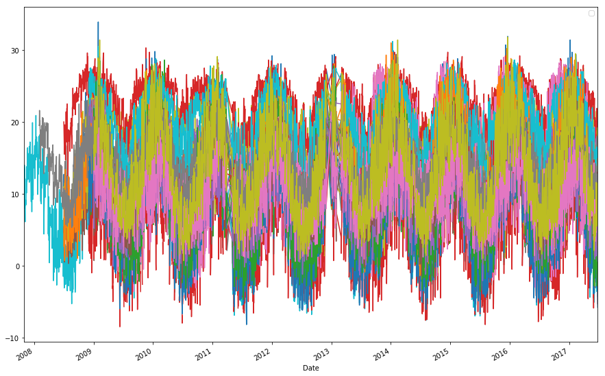
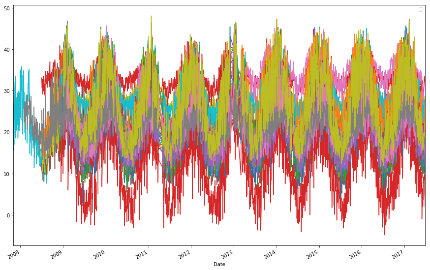
df.groupby(['Date', 'Location'])['MinTemp'].sum().unstack().plot(figsize=(15,10))
plt.legend('')
plt.show()

png

df.groupby(['Date', 'Location'])['MaxTemp'].sum().unstack().plot(figsize=(15,10))
plt.legend('')
plt.show()

png

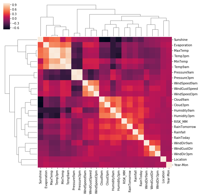
Correlation Across the Dataset

First we’ll need to convert the few categorical variables into continuous variables, we’ll do this using the basic LabelEncoder. We can then see that Rain Tomorrow appears in a cluster with RainToday, Rainfall, Humidity and Cloud.

cat_f = [x for x in df.columns if df[x].dtype == 'object']

for name in cat_f:
    enc = preprocessing.LabelEncoder()
    enc.fit(list(df[name].values.astype('str')) + list(df[name].values.astype('str')))
    df[name] = enc.transform(df[name].values.astype('str'))

sns.clustermap(df.corr())
plt.show()

png

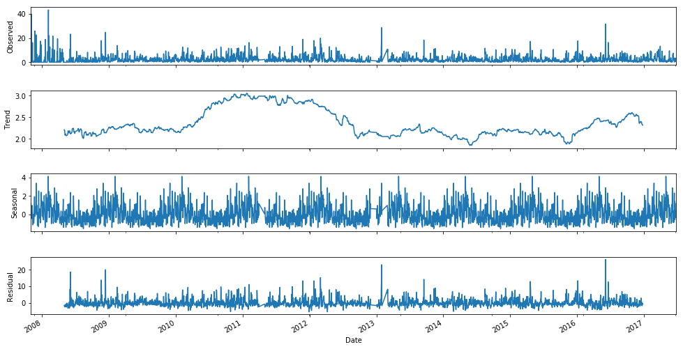
Time-Series Decomposition

import statsmodels.api as sm  
from statsmodels.tsa.stattools import acf  
from statsmodels.tsa.stattools import pacf
from statsmodels.tsa.seasonal import seasonal_decompose

C:\Users\Clint_PC\Anaconda3\lib\site-packages\statsmodels\compat\pandas.py:56: FutureWarning: The pandas.core.datetools module is deprecated and will be removed in a future version. Please use the pandas.tseries module instead.
  from pandas.core import datetools

decomposition = seasonal_decompose(df.groupby(['Date'])['Rainfall'].mean(), freq=365)  
fig = plt.figure(figsize=(15,10))  
fig = decomposition.plot()  
fig.set_size_inches(15, 8)
plt.show()

<matplotlib.figure.Figure at 0x2b033f34c50>

png

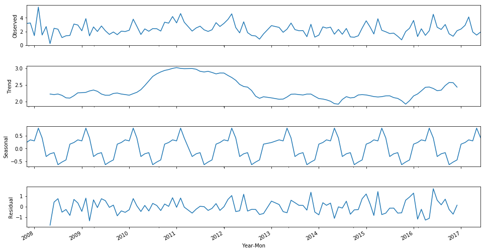
year_mon_avg = df.groupby(['Year-Mon'])['Rainfall'].mean()
year_mon_avg.index = pd.to_datetime(year_mon_avg.index)


decomposition = seasonal_decompose(year_mon_avg, freq=12)  
fig = plt.figure(figsize=(15,10))  
fig = decomposition.plot()  
fig.set_size_inches(15, 8)
plt.show()

<matplotlib.figure.Figure at 0x2b033c596a0>

png

decomposition = seasonal_decompose(df.loc[df.Location == 'Sydney'].groupby(['Date'])['Rainfall'].sum().dropna(), freq=365)  
fig = plt.figure(figsize=(15,10))  
fig = decomposition.plot()  
fig.set_size_inches(15, 8)
plt.show()

<matplotlib.figure.Figure at 0x2b03726b4e0>

png

Feature Selection

#Preprocessing
from sklearn import preprocessing
from sklearn.model_selection import train_test_split
from sklearn.preprocessing import StandardScaler

#Algos
from sklearn.linear_model import LogisticRegression
from sklearn.neighbors import KNeighborsClassifier
from sklearn.ensemble import RandomForestClassifier
from sklearn.svm import SVC
from xgboost import XGBClassifier

#Postprocessing
from sklearn.feature_selection import SelectFromModel
from sklearn.metrics import accuracy_score
from xgboost import plot_importance

C:\Users\Clint_PC\Anaconda3\lib\site-packages\sklearn\cross_validation.py:41: DeprecationWarning: This module was deprecated in version 0.18 in favor of the model_selection module into which all the refactored classes and functions are moved. Also note that the interface of the new CV iterators are different from that of this module. This module will be removed in 0.20.
  "This module will be removed in 0.20.", DeprecationWarning)

cat_f = [x for x in df.columns if df[x].dtype == 'object']

for name in cat_f:
    enc = preprocessing.LabelEncoder()
    enc.fit(list(df[name].values.astype('str')) + list(df[name].values.astype('str')))
    df[name] = enc.transform(df[name].values.astype('str'))

X_train = df.drop(['Date','RainTomorrow', 'Year-Mon', 'RISK_MM'], axis=1)
y_train = df['RainTomorrow']

X_train.fillna(-1000, inplace=True)
# our test dataset doesn't have a target variable, so we'll have to test on the train df using holdout
x_train, x_test, y_train, y_test = train_test_split(X_train, y_train, test_size=0.2)

clf3 = XGBClassifier()
clf3.fit(x_train, y_train)
print("XGBoost Score = ", clf3.score(x_test, y_test))

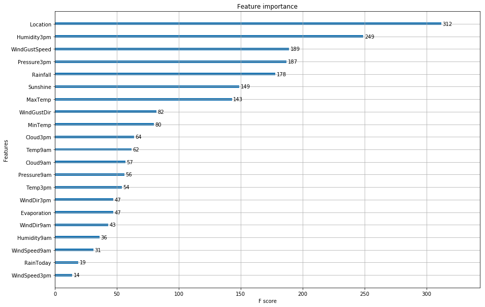
As expected above, location, humidity and pressure all appear at the top of the feature importance range!

ax = plot_importance(clf3)
fig = ax.figure
fig.set_size_inches(15, 10)
plt.show()

png

Deep Learning

#credit for help: https://machinelearningmastery.com/multivariate-time-series-forecasting-lstms-keras/

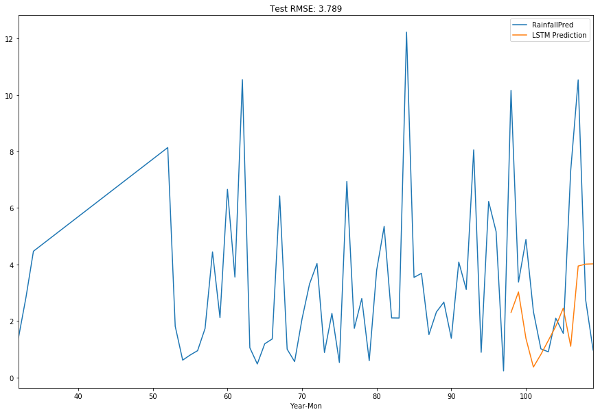
We’ll show just how easy using Keras is to build an LSTM model, train it and then use it to forecast our variables. This process highlights how easy it is to just use and abuse a model without actually understanding what’s going on, use with care!

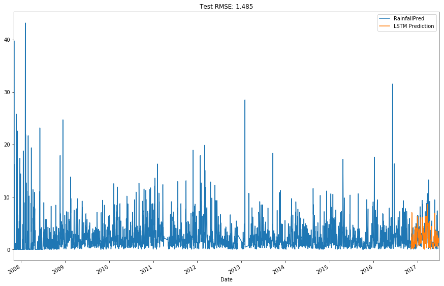
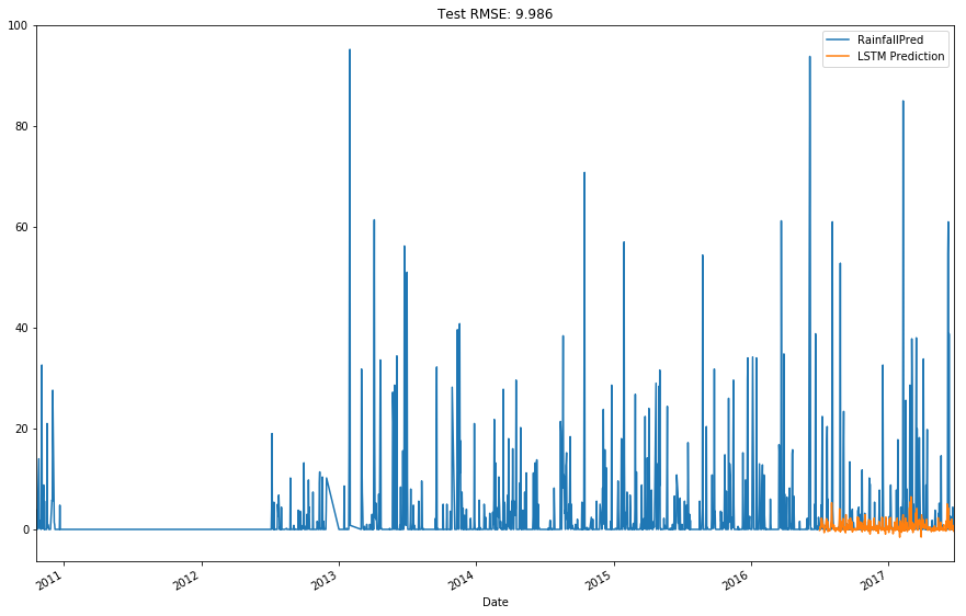
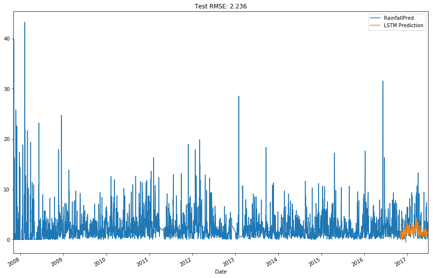
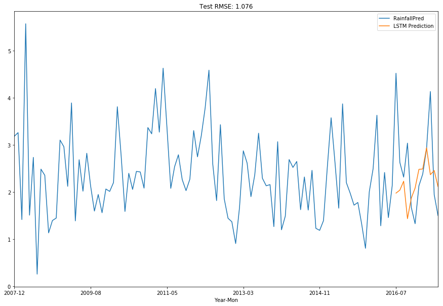
The conclusion is that it’s quite difficult to predict rainfall tomorrow based on using only variables from the previous day, as we don’t seem to be able to pick up the large swings that tend to occur. However, if we bring in current day variables, our forecast accuracy increases substantially. What this suggests is that there is likely a set of conditions which exist to cause rainfall and when these all simultaneously occur, we get the magic of rain. This is when things like humidity/pressure/cloud/wind speed all play in, as they all tie into the properties of water and impact on weather patterns.

from sklearn.preprocessing import MinMaxScaler
from sklearn.metrics import mean_squared_error
from sklearn.model_selection import train_test_split
from sklearn.metrics import mean_squared_error

from keras.models import Sequential
from keras.layers import Dense
from keras.layers import LSTM

#credit to machine learning mastery
#https://machinelearningmastery.com/multivariate-time-series-forecasting-lstms-keras/

# convert series to supervised learning
def series_to_supervised(data, n_in=1, n_out=1, dropnan=True):
    n_vars = 1 if type(data) is list else data.shape[1]
    df = pd.DataFrame(data)
    cols, names = list(), list()
    # input sequence (t-n, ... t-1)
    for i in range(n_in, 0, -1):
        cols.append(df.shift(i))
        names += [('var%d(t-%d)' % (j+1, i)) for j in range(n_vars)]
    # forecast sequence (t, t+1, ... t+n)
    for i in range(0, n_out):
        cols.append(df.shift(-i))
        if i == 0:
            names += [('var%d(t)' % (j+1)) for j in range(n_vars)]
        else:
            names += [('var%d(t+%d)' % (j+1, i)) for j in range(n_vars)]
    # put it all together
    agg = pd.concat(cols, axis=1)
    agg.columns = names
    # drop rows with NaN values
    if dropnan:
        agg.dropna(inplace=True)
    return agg

Predicting Using Only Historical Variables

def run_preds_city(df, city, groupby='Date'):
    
    df = df.loc[df['Location'] == city]
    
    cat_f = [x for x in df.columns if df[x].dtype == 'object']

    for name in cat_f:
        enc = preprocessing.LabelEncoder()
        enc.fit(list(df[name].values.astype('str')) + list(df[name].values.astype('str')))
        df[name] = enc.transform(df[name].values.astype('str'))

    
    combined_df = df.groupby([groupby]).mean()
    combined_df['RainfallPred'] = combined_df['Rainfall'].shift(1)
    combined_df.drop(['Rainfall'], axis=1, inplace=True)
    #combined_df = combined_df[['Humidity3pm', 'WindGustSpeed', 'Pressure3pm', 'Sunshine', 'MaxTemp', 'WindGustDir', 'MinTemp', 'Rainfall']]

    lstm_dataset = combined_df.values
    lstm_dataset = lstm_dataset.astype('float32')

    reframed = combined_df
    reframed.dropna(inplace=True)
    column_names = reframed.columns

    # normalize the dataset
    scaler = MinMaxScaler(feature_range=(-1, 1))
    reframed = scaler.fit_transform(reframed)

    # frame as supervised learning
    reframed = pd.DataFrame(reframed, columns=column_names)

    # split into train and test sets# split
    values = reframed.values
    forecast_period = np.round(len(values)*0.8, 0).astype(int)
    train = values[:forecast_period, :]
    test = values[forecast_period:, :]

    # split into input and outputs
    train_X, train_y = train[:, :-1], train[:, -1]
    test_X, test_y = test[:, :-1], test[:, -1]

    # reshape input to be 3D [samples, timesteps, features]
    train_X = train_X.reshape((train_X.shape[0], 1, train_X.shape[1]))
    test_X = test_X.reshape((test_X.shape[0], 1, test_X.shape[1]))

    # design network
    lstm_model = Sequential()
    lstm_model.add(LSTM(50, input_shape=(train_X.shape[1], train_X.shape[2])))
    lstm_model.add(Dense(1))
    lstm_model.compile(loss='mae', optimizer='adam')
    # fit network
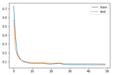
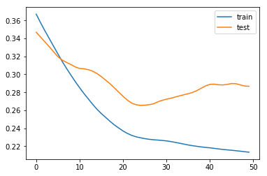
    history = lstm_model.fit(train_X, train_y, epochs=50, batch_size=72, validation_data=(test_X, test_y), verbose=0, shuffle=False)

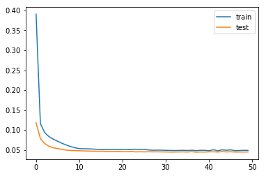
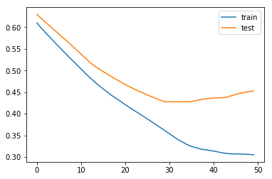
    # plot history
    plt.plot(history.history['loss'], label='train')
    plt.plot(history.history['val_loss'], label='test')
    plt.legend()
    plt.show()
    
    # make a prediction
    yhat = lstm_model.predict(test_X)

    #to reverse MinMax reshape based on original shape
    test_X = test_X.reshape((test_X.shape[0], test_X.shape[2]))
    # invert scaling for forecast
    inv_yhat = np.concatenate((test_X[:, 0:], yhat), axis=1)
    inv_yhat = scaler.inverse_transform(inv_yhat)
    inv_yhat = inv_yhat[:,-1]
    # invert scaling for actual
    test_y = test_y.reshape((len(test_y), 1))
    inv_y = np.concatenate((test_X[:,0:], test_y), axis=1)
    inv_y = scaler.inverse_transform(inv_y)
    inv_y = inv_y[:,-1]
    # calculate RMSE
    rmse = np.sqrt(mean_squared_error(inv_y, inv_yhat))
    rmse_title_lstm = 'Test RMSE: %.3f' % rmse
    
    
    lstm_predictions = [np.nan for _ in range(0,len(train_X))]
    combined_df['LSTM Prediction'] = lstm_predictions + list(inv_yhat)
    combined_df[['RainfallPred', 'LSTM Prediction']].plot( figsize=(15,10), title=rmse_title_lstm)
    plt.show()

def run_preds(df, forecast_period, groupby='Date'):
    
    combined_df = df.groupby([groupby]).mean()
    combined_df['RainfallPred'] = combined_df['Rainfall'].shift(1)
    combined_df.drop(['Rainfall'], axis=1, inplace=True)
    #combined_df = combined_df[['Humidity3pm', 'WindGustSpeed', 'Pressure3pm', 'Sunshine', 'MaxTemp', 'WindGustDir', 'MinTemp', 'Rainfall']]

    lstm_dataset = combined_df.values
    lstm_dataset = lstm_dataset.astype('float32')

    reframed = combined_df
    reframed.dropna(inplace=True)
    column_names = reframed.columns

    # normalize the dataset
    scaler = MinMaxScaler(feature_range=(-1, 1))
    reframed = scaler.fit_transform(reframed)

    # frame as supervised learning
    reframed = pd.DataFrame(reframed, columns=column_names)

    # split into train and test sets# split  
    values = reframed.values
    train = values[:forecast_period, :]
    test = values[forecast_period:, :]

    # split into input and outputs
    train_X, train_y = train[:, :-1], train[:, -1]
    test_X, test_y = test[:, :-1], test[:, -1]

    # reshape input to be 3D [samples, timesteps, features]
    train_X = train_X.reshape((train_X.shape[0], 1, train_X.shape[1]))
    test_X = test_X.reshape((test_X.shape[0], 1, test_X.shape[1]))

    # design network
    lstm_model = Sequential()
    lstm_model.add(LSTM(50, input_shape=(train_X.shape[1], train_X.shape[2])))
    lstm_model.add(Dense(1))
    lstm_model.compile(loss='mae', optimizer='adam')
    # fit network
    history = lstm_model.fit(train_X, train_y, epochs=50, batch_size=72, validation_data=(test_X, test_y), verbose=0, shuffle=False)

    # plot history
    plt.plot(history.history['loss'], label='train')
    plt.plot(history.history['val_loss'], label='test')
    plt.legend()
    plt.show()
    
    # make a prediction
    yhat = lstm_model.predict(test_X)

    #to reverse MinMax reshape based on original shape
    test_X = test_X.reshape((test_X.shape[0], test_X.shape[2]))
    # invert scaling for forecast
    inv_yhat = np.concatenate((test_X[:, 0:], yhat), axis=1)
    inv_yhat = scaler.inverse_transform(inv_yhat)
    inv_yhat = inv_yhat[:,-1]
    # invert scaling for actual
    test_y = test_y.reshape((len(test_y), 1))
    inv_y = np.concatenate((test_X[:,0:], test_y), axis=1)
    inv_y = scaler.inverse_transform(inv_y)
    inv_y = inv_y[:,-1]
    # calculate RMSE
    rmse = np.sqrt(mean_squared_error(inv_y, inv_yhat))
    rmse_title_lstm = 'Test RMSE: %.3f' % rmse
    
    
    lstm_predictions = [np.nan for _ in range(0,len(train_X))]
    combined_df['LSTM Prediction'] = lstm_predictions + list(inv_yhat)
    combined_df[['RainfallPred', 'LSTM Prediction']].plot( figsize=(15,10), title=rmse_title_lstm)
    plt.show()

run_preds_city(df, 'Sydney', 'Year-Mon')

C:\Users\Clint_PC\Anaconda3\lib\site-packages\ipykernel\__main__.py:10: SettingWithCopyWarning: 
A value is trying to be set on a copy of a slice from a DataFrame.
Try using .loc[row_indexer,col_indexer] = value instead

See the caveats in the documentation: http://pandas.pydata.org/pandas-docs/stable/indexing.html#indexing-view-versus-copy

png

run_preds_city(df, 'Sydney', 'Date')

C:\Users\Clint_PC\Anaconda3\lib\site-packages\ipykernel\__main__.py:10: SettingWithCopyWarning: 
A value is trying to be set on a copy of a slice from a DataFrame.
Try using .loc[row_indexer,col_indexer] = value instead

See the caveats in the documentation: http://pandas.pydata.org/pandas-docs/stable/indexing.html#indexing-view-versus-copy

png

run_preds(df, 3200, 'Date')

png

run_preds(df, 100, 'Year-Mon')

png

Predicting Using Current Days Variables

def run_preds_supervised(df, forecast_period, groupby='Date'):
    
    combined_df = df.groupby([groupby]).mean()
    #combined_df = combined_df[['Humidity3pm', 'WindGustSpeed', 'Pressure3pm', 'Sunshine', 'MaxTemp', 'WindGustDir', 'MinTemp', 'Rainfall']]
    combined_df['RainfallPred'] = combined_df['Rainfall'].shift(1)
    combined_df.drop(['Rainfall'], axis=1, inplace=True)
    combined_df.dropna(inplace=True)
    lstm_dataset = combined_df.values
    lstm_dataset = lstm_dataset.astype('float32')
    
    reframed = series_to_supervised(lstm_dataset, 1, 1)

    column_names = reframed.columns

    # normalize the dataset
    scaler = MinMaxScaler(feature_range=(-1, 1))
    reframed = scaler.fit_transform(reframed)

    # frame as supervised learning
    reframed = pd.DataFrame(reframed, columns=column_names)

    # split into train and test sets# split  
    values = reframed.values
    train = values[:forecast_period, :]
    test = values[forecast_period:, :]

    # split into input and outputs
    train_X, train_y = train[:, :-1], train[:, -1]
    test_X, test_y = test[:, :-1], test[:, -1]

    # reshape input to be 3D [samples, timesteps, features]
    train_X = train_X.reshape((train_X.shape[0], 1, train_X.shape[1]))
    test_X = test_X.reshape((test_X.shape[0], 1, test_X.shape[1]))

    
    # design network
    lstm_model = Sequential()
    lstm_model.add(LSTM(50, input_shape=(train_X.shape[1], train_X.shape[2])))
    lstm_model.add(Dense(1))
    lstm_model.compile(loss='mae', optimizer='adam')
    # fit network
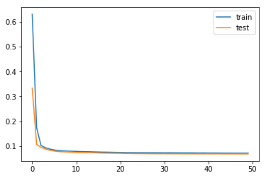
    history = lstm_model.fit(train_X, train_y, epochs=50, batch_size=72, validation_data=(test_X, test_y), verbose=0, shuffle=False)

    # plot history
    plt.plot(history.history['loss'], label='train')
    plt.plot(history.history['val_loss'], label='test')
    plt.legend()
    plt.show()
    
    
    # make a prediction
    yhat = lstm_model.predict(test_X)

    #to reverse MinMax reshape based on original shape
    test_X = test_X.reshape((test_X.shape[0], test_X.shape[2]))
    # invert scaling for forecast
    inv_yhat = np.concatenate((test_X[:, 0:], yhat), axis=1)
    inv_yhat = scaler.inverse_transform(inv_yhat)
    inv_yhat = inv_yhat[:,-1]
    # invert scaling for actual
    test_y = test_y.reshape((len(test_y), 1))
    inv_y = np.concatenate((test_X[:,0:], test_y), axis=1)
    inv_y = scaler.inverse_transform(inv_y)
    inv_y = inv_y[:,-1]
    # calculate RMSE
    rmse = np.sqrt(mean_squared_error(inv_y, inv_yhat))
    rmse_title_lstm = 'Test RMSE: %.3f' % rmse
    
    
    lstm_predictions = [np.nan for _ in range(0,len(train_X)+1)]
    combined_df['LSTM Prediction'] = lstm_predictions + list(inv_yhat)
    combined_df[['RainfallPred', 'LSTM Prediction']].plot( figsize=(15,10), title=rmse_title_lstm)
    plt.show()

run_preds_supervised(df, 3200, 'Date')

png