Global Economic Trade Data
With Global tensions increasing among the looming trade war, let’s take a deep dive into historical trade statistics from the UN and see who really is a net exporter/net importer, as well as where the trade values primarily lie. Data sourced from the UN here
import pandas as pd
import numpy as np
import matplotlib.pyplot as plt
import matplotlib.ticker as mtick

import seaborn as sns
import plotly.plotly as py
df = pd.read_csv(r"D:\Downloads\commodity_trade_statistics_data.csv\commodity_trade_statistics_data.csv")
C:\Users\Clint_PC\Anaconda3\lib\site-packages\IPython\core\interactiveshell.py:2698: DtypeWarning:

Columns (2) have mixed types. Specify dtype option on import or set low_memory=False.
df.head()
| country_or_area | year | comm_code | commodity | flow | trade_usd | weight_kg | quantity_name | quantity | category | |
|---|---|---|---|---|---|---|---|---|---|---|
| 0 | Afghanistan | 2016 | 10410 | Sheep, live | Export | 6088 | 2339.0 | Number of items | 51.0 | 01_live_animals |
| 1 | Afghanistan | 2016 | 10420 | Goats, live | Export | 3958 | 984.0 | Number of items | 53.0 | 01_live_animals |
| 2 | Afghanistan | 2008 | 10210 | Bovine animals, live pure-bred breeding | Import | 1026804 | 272.0 | Number of items | 3769.0 | 01_live_animals |
| 3 | Albania | 2016 | 10290 | Bovine animals, live, except pure-bred breeding | Import | 2414533 | 1114023.0 | Number of items | 6853.0 | 01_live_animals |
| 4 | Albania | 2016 | 10392 | Swine, live except pure-bred breeding > 50 kg | Import | 14265937 | 9484953.0 | Number of items | 96040.0 | 01_live_animals |
df.info()
<class 'pandas.core.frame.DataFrame'>
RangeIndex: 8225871 entries, 0 to 8225870
Data columns (total 10 columns):
country_or_area    object
year               int64
comm_code          object
commodity          object
flow               object
trade_usd          int64
weight_kg          float64
quantity_name      object
quantity           float64
category           object
dtypes: float64(2), int64(2), object(6)
memory usage: 627.6+ MB
Basic Exploration
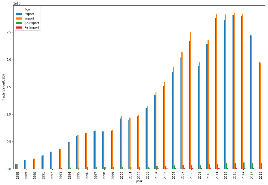
We have a dataset from 1988-2016, which is quite large but pretty simplistic setup. If we look at a time aggregate, we see the global increase to 2014, but recently the drop-off of 2015/2016. This could just be a data issue, but perhaps global trade has been slowing down…
np.unique(df.year)
array([1988, 1989, 1990, 1991, 1992, 1993, 1994, 1995, 1996, 1997, 1998,
       1999, 2000, 2001, 2002, 2003, 2004, 2005, 2006, 2007, 2008, 2009,
       2010, 2011, 2012, 2013, 2014, 2015, 2016], dtype=int64)
df.groupby(['year', 'flow'])['trade_usd'].sum().unstack().plot(kind='bar', figsize=(15,10))
plt.ylabel('Trade Value(USD)')
plt.show()
country_flows = df.groupby(['country_or_area', 'flow'])['trade_usd'].sum().unstack()
country_flows.fillna(0, inplace=True)

country_flows['Export'] = country_flows['Export'] + country_flows['Re-Export']
country_flows['Import'] = country_flows['Import'] + country_flows['Re-Import']
country_flows.drop(['Re-Export', 'Re-Import'], axis=1, inplace=True)

country_flows['Delta'] = country_flows['Export'] - country_flows['Import']
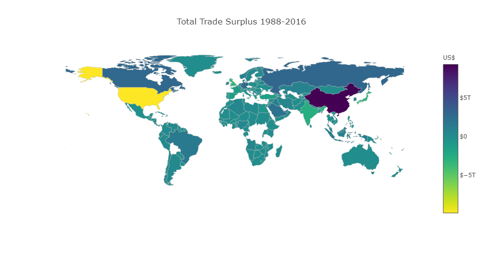
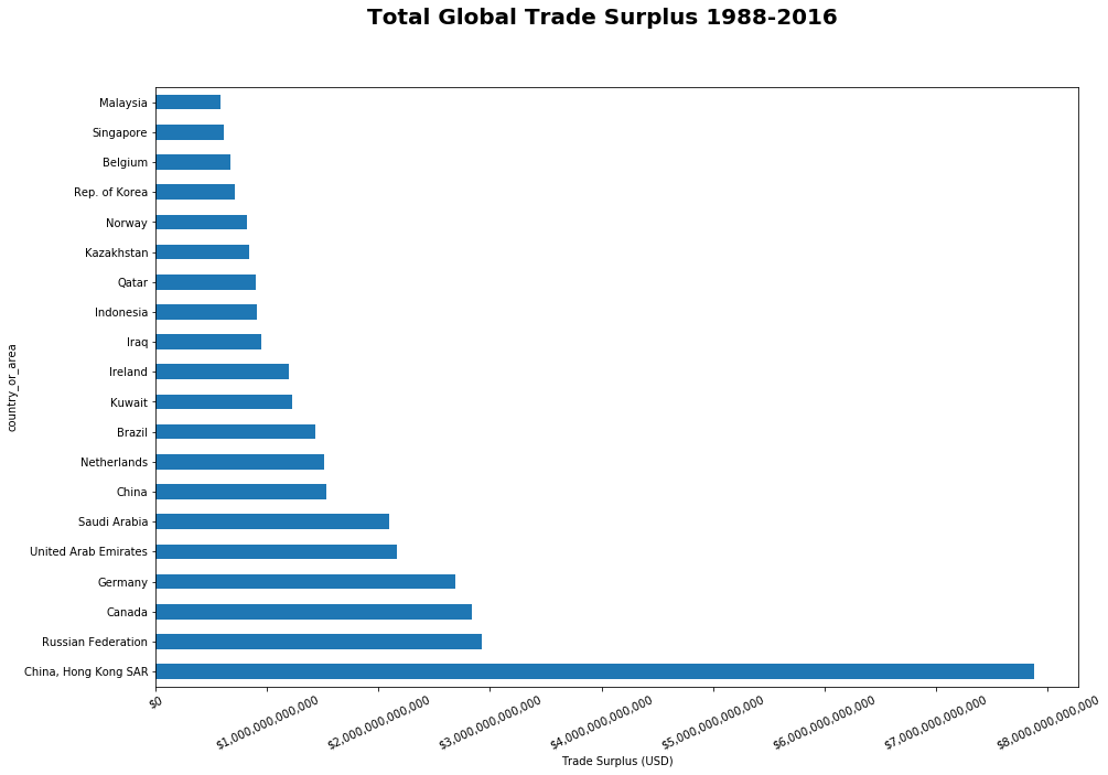
Surplus
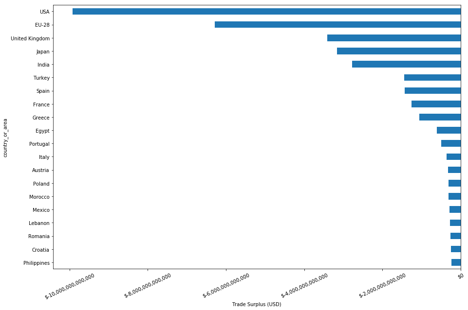
The hot topic, global trade surplus. Evidently, the USA has indeed been copping it quite bad since 1988, with a total trade deficit over over USD10T, whilst China is enjoying the other end of that with a positive surplus of almost USD8T.
df_codes = pd.read_csv('https://raw.githubusercontent.com/plotly/datasets/master/2014_world_gdp_with_codes.csv')
df_codes.set_index(['COUNTRY'], inplace=True)

country_flows_merged = country_flows.merge(df_codes, how='left', left_index=True, right_index=True)
country_flows_merged.loc[country_flows_merged.index == 'USA', 'CODE'] = 'USA'
country_flows_merged.loc[country_flows_merged.index == 'China, Hong Kong SAR', 'CODE'] = 'CHN'
country_flows_merged.loc[country_flows_merged.index == 'China, Macao SAR', 'CODE'] = 'CHN'
country_flows_merged.loc[country_flows_merged.index == 'Russian Federation', 'CODE'] = 'RUS'
country_flows_merged.loc[country_flows_merged.index == 'Bahamams', 'CODE'] = 'BHM'
country_flows_merged.loc[country_flows_merged.index == 'Viet Nam', 'CODE'] = 'VNM'
country_flows_merged.loc[country_flows_merged.index == 'Rep. of Korea', 'CODE'] = 'KOR'

country_flows_merged_clean = pd.DataFrame(country_flows_merged.groupby(['CODE'])['Delta'].sum())
data = [ dict(
        type = 'choropleth',
        locations = country_flows_merged_clean.index,
        z = country_flows_merged_clean['Delta'],
        colorscale = 'Viridis',
        autocolorscale = False,
        reversescale = True,
        marker = dict(
            line = dict (
                color = 'rgb(180,180,180)',
                width = 0.5
            ) ),
        colorbar = dict(
            autotick = False,
            tickprefix = '$',
            title = 'US$'),
      ) ]

layout = dict(
    title = 'Total Trade Surplus 1988-2016',
    geo = dict(
        showframe = False,
        showcoastlines = False,
        projection = dict(
            type = 'Mercator'
        )
    )
)

fig = dict( data=data, layout=layout )
py.iplot( fig, validate=False, filename='d3-world-map' )
fig, ax = plt.subplots(1,1)
plt.suptitle('Total Global Trade Surplus 1988-2016', size=20, fontweight='bold')
country_flows['Delta'].sort_values(ascending=False).head(20).plot(kind='barh', figsize=(15,10))
plt.xlabel('Trade Surplus (USD)')
fmt = '${x:,.0f}'
tick = mtick.StrMethodFormatter(fmt)
ax.xaxis.set_major_formatter(tick)
plt.xticks(rotation=25)
plt.show()

fig, ax = plt.subplots(1,1)

country_flows['Delta'].sort_values(ascending=False).tail(20).plot(kind='barh', figsize=(15,10))
plt.xlabel('Trade Surplus (USD)')
tick = mtick.StrMethodFormatter(fmt)
ax.xaxis.set_major_formatter(tick)
plt.xticks(rotation=25)
plt.show()
country_ts = df.groupby(['country_or_area', 'year', 'flow'])['trade_usd'].sum().unstack()
country_ts.fillna(0, inplace=True)
country_ts['Export'] = country_ts['Export'] + country_ts['Re-Export']
country_ts['Import'] = country_ts['Import'] + country_ts['Re-Import']
country_ts.drop(['Re-Export', 'Re-Import'], axis=1, inplace=True)
country_ts['Surplus'] = country_ts['Export'] - country_ts['Import']

country_ts = country_ts['Surplus']
country_ts = country_ts.unstack().T
country_ts.fillna(0, inplace=True)
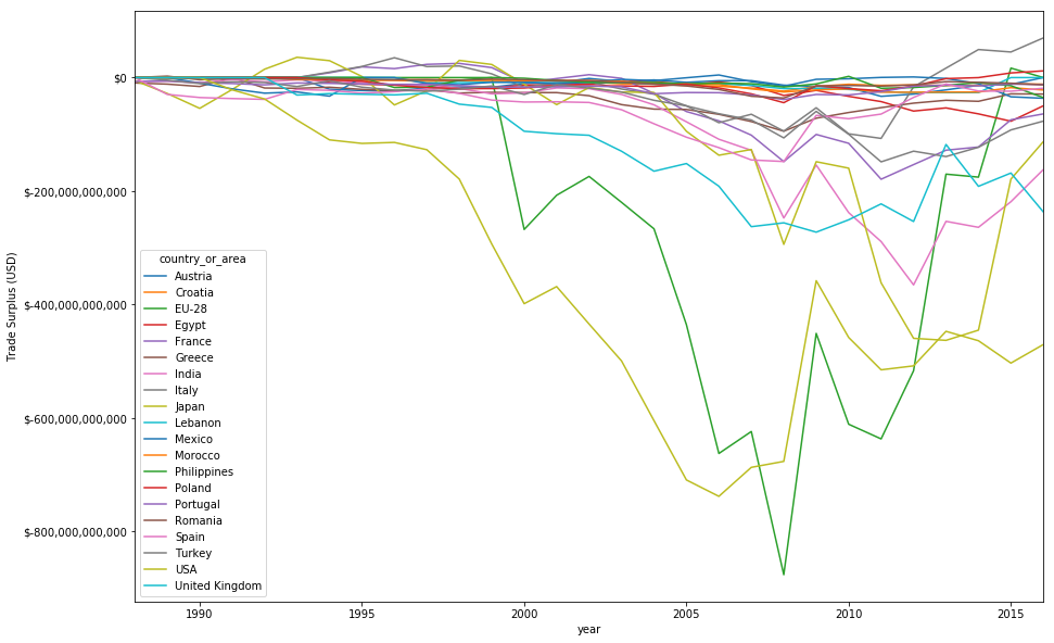
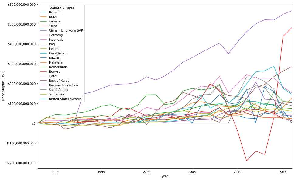
country_ordered = country_ts.mean(axis=0).sort_values().index
top_20 = country_ordered[0:20]
bottom_20 = country_ordered[-20:]
fig, ax = plt.subplots(1,1)
country_ts.loc[:, country_ts.columns.isin(top_20)].plot(figsize=(15,10),ax=ax)
fmt = '${x:,.0f}'
plt.ylabel('Trade Surplus (USD)')
tick = mtick.StrMethodFormatter(fmt)
ax.yaxis.set_major_formatter(tick)
plt.show()


fig, ax = plt.subplots(1,1)
country_ts.loc[:, country_ts.columns.isin(bottom_20)].plot(figsize=(15,10), ax=ax)
fmt = '${x:,.0f}'
tick = mtick.StrMethodFormatter(fmt)
ax.yaxis.set_major_formatter(tick)
plt.ylabel('Trade Surplus (USD)')
plt.show()
country_ts
| country_or_area | Afghanistan | Albania | Algeria | Andorra | Angola | Anguilla | Antigua and Barbuda | Argentina | Armenia | Aruba | ... | United Kingdom | United Rep. of Tanzania | Uruguay | Vanuatu | Venezuela | Viet Nam | Wallis and Futuna Isds | Yemen | Zambia | Zimbabwe |
|---|---|---|---|---|---|---|---|---|---|---|---|---|---|---|---|---|---|---|---|---|---|
| year | |||||||||||||||||||||
| 1988 | 0.000000e+00 | 0.000000e+00 | 0.000000e+00 | 0.000000e+00 | 0.000000e+00 | 0.0 | 0.000000e+00 | 0.000000e+00 | 0.000000e+00 | 0.000000e+00 | ... | 0.000000e+00 | 0.000000e+00 | 0.000000e+00 | 0.0 | 0.000000e+00 | 0.000000e+00 | 0.0 | 0.000000e+00 | 0.000000e+00 | 0.000000e+00 |
| 1989 | 0.000000e+00 | 0.000000e+00 | 0.000000e+00 | 0.000000e+00 | 0.000000e+00 | 0.0 | 0.000000e+00 | 0.000000e+00 | 0.000000e+00 | 0.000000e+00 | ... | 0.000000e+00 | 0.000000e+00 | 0.000000e+00 | 0.0 | 0.000000e+00 | 0.000000e+00 | 0.0 | 0.000000e+00 | 0.000000e+00 | 0.000000e+00 |
| 1990 | 0.000000e+00 | 0.000000e+00 | 0.000000e+00 | 0.000000e+00 | 0.000000e+00 | 0.0 | 0.000000e+00 | 0.000000e+00 | 0.000000e+00 | 0.000000e+00 | ... | 0.000000e+00 | 0.000000e+00 | 0.000000e+00 | 0.0 | 0.000000e+00 | 0.000000e+00 | 0.0 | 0.000000e+00 | 0.000000e+00 | 0.000000e+00 |
| 1991 | 0.000000e+00 | 0.000000e+00 | 0.000000e+00 | 0.000000e+00 | 0.000000e+00 | 0.0 | 0.000000e+00 | 0.000000e+00 | 0.000000e+00 | 0.000000e+00 | ... | 0.000000e+00 | 0.000000e+00 | 0.000000e+00 | 0.0 | 0.000000e+00 | 0.000000e+00 | 0.0 | 0.000000e+00 | 0.000000e+00 | 0.000000e+00 |
| 1992 | 0.000000e+00 | 0.000000e+00 | 4.977971e+09 | 0.000000e+00 | 0.000000e+00 | 0.0 | 0.000000e+00 | 0.000000e+00 | 0.000000e+00 | 0.000000e+00 | ... | 0.000000e+00 | 0.000000e+00 | 0.000000e+00 | 0.0 | 0.000000e+00 | 0.000000e+00 | 0.0 | 0.000000e+00 | 0.000000e+00 | 0.000000e+00 |
| 1993 | 0.000000e+00 | 0.000000e+00 | 2.624781e+09 | 0.000000e+00 | 0.000000e+00 | 0.0 | 0.000000e+00 | -7.310326e+09 | 0.000000e+00 | 0.000000e+00 | ... | -3.083832e+10 | 0.000000e+00 | 0.000000e+00 | -72155394.0 | 0.000000e+00 | 0.000000e+00 | 0.0 | 0.000000e+00 | 0.000000e+00 | 0.000000e+00 |
| 1994 | 0.000000e+00 | 0.000000e+00 | -2.009735e+09 | 0.000000e+00 | 0.000000e+00 | 0.0 | 0.000000e+00 | -1.148480e+10 | 0.000000e+00 | 0.000000e+00 | ... | -2.823188e+10 | 0.000000e+00 | -6.635727e+08 | -61435785.0 | 7.780871e+09 | 0.000000e+00 | 0.0 | 0.000000e+00 | 0.000000e+00 | 0.000000e+00 |
| 1995 | 0.000000e+00 | 0.000000e+00 | -2.851504e+09 | -1.955355e+09 | 0.000000e+00 | 0.0 | 0.000000e+00 | 1.681868e+09 | 0.000000e+00 | 0.000000e+00 | ... | -2.943779e+10 | -1.802217e+09 | -5.340502e+08 | 0.0 | 7.491302e+09 | 0.000000e+00 | 0.0 | 0.000000e+00 | 2.885883e+08 | -2.329738e+08 |
| 1996 | 0.000000e+00 | -1.454683e+09 | 3.987253e+09 | -2.030231e+09 | 0.000000e+00 | 0.0 | 0.000000e+00 | 9.614470e+07 | 0.000000e+00 | 0.000000e+00 | ... | -3.051357e+10 | -1.386921e+09 | -7.044310e+08 | 0.0 | 1.358184e+10 | 0.000000e+00 | 0.0 | 0.000000e+00 | 1.050435e+08 | 0.000000e+00 |
| 1997 | 0.000000e+00 | -9.826906e+08 | 1.041153e+10 | -2.026583e+09 | 0.000000e+00 | 0.0 | 0.000000e+00 | -7.837164e+09 | -1.078332e+09 | 0.000000e+00 | ... | -2.764686e+10 | -7.871056e+08 | -6.943273e+08 | 0.0 | 9.099637e+09 | 0.000000e+00 | 0.0 | 0.000000e+00 | 9.573334e+07 | 0.000000e+00 |
| 1998 | 0.000000e+00 | -1.267205e+09 | 8.703141e+08 | -2.012552e+09 | 0.000000e+00 | 0.0 | 0.000000e+00 | -9.887151e+09 | 0.000000e+00 | 0.000000e+00 | ... | -4.685271e+10 | -1.224130e+09 | -7.568320e+08 | 0.0 | 2.139015e+09 | 0.000000e+00 | 0.0 | 0.000000e+00 | -1.021526e+08 | 0.000000e+00 |
| 1999 | 0.000000e+00 | -1.606507e+09 | 6.726863e+09 | -2.072000e+09 | 0.000000e+00 | 0.0 | -6.588974e+08 | -4.350568e+09 | -1.158361e+09 | 0.000000e+00 | ... | -5.267369e+10 | -1.039648e+09 | -9.777869e+08 | 0.0 | 5.648073e+09 | 0.000000e+00 | 0.0 | 0.000000e+00 | 3.783235e+08 | 0.000000e+00 |
| 2000 | 0.000000e+00 | -1.655984e+09 | 2.575842e+10 | -1.933261e+09 | 0.000000e+00 | -181025753.0 | -5.923397e+08 | 2.121131e+09 | -9.119766e+08 | -1.324461e+09 | ... | -9.469960e+10 | -1.037134e+09 | -1.096083e+09 | -63454919.0 | 1.533502e+10 | -9.734810e+08 | -41836489.0 | 0.000000e+00 | 3.459299e+07 | 2.853201e+09 |
| 2001 | 0.000000e+00 | -2.051401e+09 | 1.840103e+10 | -1.979289e+09 | 0.000000e+00 | -149007477.0 | 0.000000e+00 | 1.257786e+10 | -7.622534e+08 | -1.374757e+09 | ... | -9.899567e+10 | -1.015586e+09 | -8.997630e+08 | 0.0 | 7.780487e+09 | -7.759209e+08 | -36810946.0 | 0.000000e+00 | -8.014222e+07 | 2.664529e+08 |
| 2002 | 0.000000e+00 | -2.346887e+09 | 1.364481e+10 | -2.271637e+09 | 0.000000e+00 | -131097857.0 | 0.000000e+00 | 3.343965e+10 | -6.625938e+08 | -1.429234e+09 | ... | -1.018208e+11 | -7.483888e+08 | -2.786970e+07 | 0.0 | 1.113104e+10 | -3.016891e+09 | -42538337.0 | 0.000000e+00 | -1.643969e+08 | 6.274689e+08 |
| 2003 | 0.000000e+00 | -2.834230e+09 | 2.221645e+10 | -2.845919e+09 | 0.000000e+00 | -145075316.0 | 0.000000e+00 | 3.217596e+10 | -9.128414e+08 | -1.528860e+09 | ... | -1.299393e+11 | -1.051751e+09 | 1.418170e+08 | 0.0 | 1.585320e+10 | -5.780695e+09 | -48840794.0 | 0.000000e+00 | -6.615196e+08 | 0.000000e+00 |
| 2004 | 0.000000e+00 | -3.395818e+09 | 2.754754e+10 | -3.277072e+09 | 0.000000e+00 | -193380938.0 | 0.000000e+00 | 2.426092e+10 | -1.055779e+09 | -1.592979e+09 | ... | -1.651775e+11 | -9.325555e+08 | 5.332561e+06 | 0.0 | 2.354149e+10 | -6.238985e+09 | -59311566.0 | -4.898794e+08 | -5.215778e+08 | 2.584781e+08 |
| 2005 | 0.000000e+00 | -3.181794e+09 | 5.128971e+10 | 2.854751e+08 | 0.000000e+00 | 0.0 | -5.753043e+08 | 2.283550e+10 | -1.248564e+09 | -1.840389e+09 | ... | -1.516742e+11 | -1.283666e+09 | -2.732888e+08 | 0.0 | 3.187031e+10 | -4.354305e+09 | -58216986.0 | -5.005515e+08 | -6.459125e+08 | -3.911527e+08 |
| 2006 | 0.000000e+00 | -4.292603e+09 | 6.631373e+10 | -3.247275e+09 | 0.000000e+00 | -325322708.0 | -1.341496e+09 | 2.474384e+10 | -2.089321e+09 | -1.864738e+09 | ... | -1.916517e+11 | -2.407801e+09 | -6.420622e+08 | -131829809.0 | 2.254874e+10 | -5.619724e+09 | -68957216.0 | -1.253978e+08 | 1.088041e+09 | 5.367925e+09 |
| 2007 | 0.000000e+00 | -6.255337e+09 | 6.506391e+10 | -3.552197e+09 | 6.616588e+10 | -477438972.0 | -7.588969e+08 | 2.214508e+10 | -3.253586e+09 | -2.031968e+09 | ... | -2.630142e+11 | -3.605083e+09 | -8.337874e+08 | -190579252.0 | -5.573032e+10 | -1.616434e+10 | 0.0 | -3.419853e+09 | 8.942910e+08 | 7.071300e+08 |
| 2008 | -4.959589e+09 | -6.170419e+09 | 7.964574e+10 | -3.605889e+09 | 0.000000e+00 | -520539691.0 | 0.000000e+00 | 2.505528e+10 | -5.820556e+09 | -2.023501e+09 | ... | -2.562436e+11 | -4.739079e+09 | -2.879242e+09 | 0.0 | 3.185560e+10 | -1.911097e+10 | 0.0 | -4.352683e+09 | 4.366072e+08 | -7.750495e+08 |
| 2009 | -5.865988e+09 | -6.921291e+09 | 1.187119e+10 | -3.035165e+09 | 3.344111e+10 | 0.0 | -5.805141e+08 | 3.370385e+10 | -4.824101e+09 | -2.026905e+09 | ... | -2.727260e+11 | -3.155496e+09 | -9.029825e+08 | -274790443.0 | 1.402614e+10 | -1.478188e+10 | 0.0 | -4.479290e+09 | 8.036351e+08 | -5.403382e+08 |
| 2010 | -9.531532e+09 | -6.105691e+09 | 3.210216e+10 | -2.896375e+09 | 6.893769e+10 | 0.0 | -8.680018e+08 | 2.270652e+10 | -5.337767e+09 | -1.893021e+09 | ... | -2.509274e+11 | -3.285051e+09 | -1.327965e+09 | -268223254.0 | 3.193969e+10 | -1.504362e+10 | 0.0 | -4.292682e+09 | 1.807544e+09 | -2.188030e+09 |
| 2011 | -1.202892e+10 | -6.895292e+09 | 5.243315e+10 | -3.013561e+09 | 9.127279e+10 | 0.0 | -8.333670e+08 | 1.796716e+10 | -5.200048e+09 | -2.267178e+09 | ... | -2.228197e+11 | -5.961833e+09 | -2.302773e+09 | -256985331.0 | 6.141342e+10 | -1.226261e+10 | 0.0 | -5.084629e+09 | 1.477698e+09 | -4.255234e+09 |
| 2012 | -1.155216e+10 | -5.823821e+09 | 4.299272e+10 | -2.625897e+09 | 8.428018e+10 | 0.0 | -9.563822e+08 | 2.392374e+10 | -5.402397e+09 | -2.173487e+09 | ... | -2.539077e+11 | -5.765932e+09 | -2.179933e+09 | 0.0 | 2.799792e+10 | -2.477569e+09 | 0.0 | -6.760083e+09 | 1.586056e+08 | -2.720127e+09 |
| 2013 | -1.607888e+10 | -5.098143e+09 | 2.217633e+10 | -2.776432e+09 | 8.191293e+10 | 0.0 | -8.923109e+08 | 2.974052e+09 | -5.382683e+09 | -2.271111e+09 | ... | -1.180139e+11 | -8.135488e+09 | -2.241516e+09 | 0.0 | 3.532485e+10 | -5.268717e+09 | 0.0 | -1.216474e+10 | -4.851883e+08 | -3.144458e+09 |
| 2014 | -1.425329e+10 | -5.598497e+09 | 3.539218e+09 | -2.922535e+09 | 5.983774e+10 | 0.0 | -1.021693e+09 | 6.299247e+09 | -5.111961e+09 | -2.335870e+09 | ... | -1.918521e+11 | -6.309072e+09 | -1.016277e+09 | 0.0 | 0.000000e+00 | -3.327046e+09 | 0.0 | -1.213216e+10 | -8.110588e+08 | -2.633740e+09 |
| 2015 | -1.430292e+10 | -4.781125e+09 | -3.401424e+10 | 0.000000e+00 | 3.257998e+10 | 0.0 | -8.305295e+08 | -5.997725e+09 | -3.213331e+09 | -2.170264e+09 | ... | -1.683963e+11 | -8.295337e+09 | -1.584236e+09 | 0.0 | 0.000000e+00 | -1.166668e+10 | 0.0 | -7.844405e+09 | -1.668920e+09 | -2.688277e+09 |
| 2016 | -1.187537e+10 | -5.414345e+09 | -3.419716e+10 | 0.000000e+00 | 0.000000e+00 | 0.0 | -7.404599e+08 | 4.185648e+09 | -2.505202e+09 | -2.043652e+09 | ... | -2.370673e+11 | -2.671288e+09 | -8.270755e+08 | 0.0 | 0.000000e+00 | 0.000000e+00 | 0.0 | 0.000000e+00 | 0.000000e+00 | -1.765976e+09 |
29 rows × 209 columns
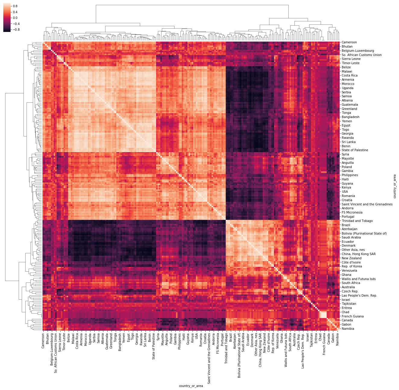
Not surprisingly, a clustermap reveals two primary clusters: net exporters and net importers.
sns.clustermap(country_ts.corr(), figsize=(20,20))
plt.show()
Valuable Trade Items
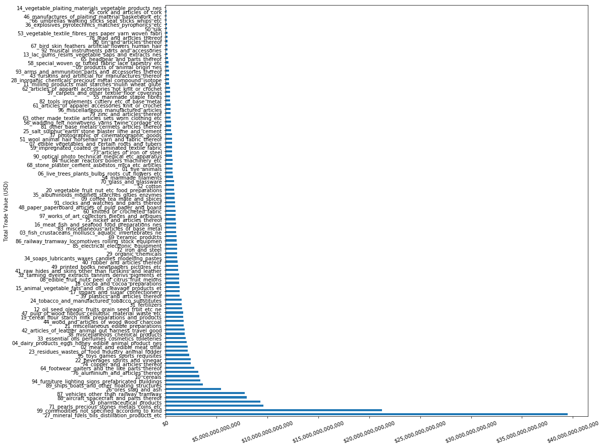
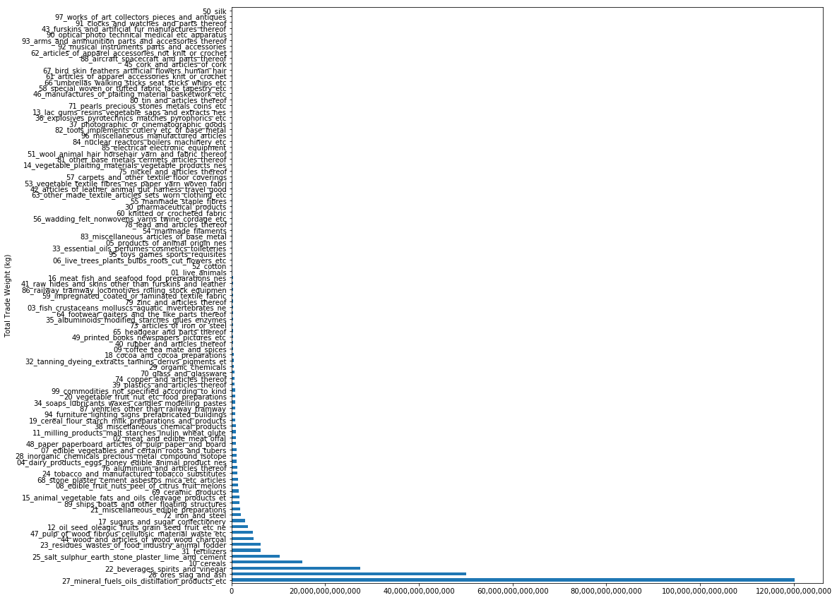
What everybody cares about… what can get you rich. Not suprisingly, the most value traded are in things like minerals/fuels/distillation products i.e. oil. What’s more interesting is when we break it down by weight as well, and look at the most valuable items on a weight basis.
fig, ax = plt.subplots()
category_value = df.loc[df.category != 'all_commodities'].groupby(['category'])['trade_usd'].sum()
category_value.sort_values(ascending=False).plot(kind='barh', figsize=(15,15), ax=ax)
fmt = '${x:,.0f}'
tick = mtick.StrMethodFormatter(fmt)
ax.xaxis.set_major_formatter(tick)
plt.xticks(rotation=20)
plt.ylabel('Total Trade Value (USD)')
plt.show()
fig, ax = plt.subplots()
category_weight = df.loc[df.category != 'all_commodities'].groupby(['category'])['weight_kg'].sum()
category_weight.sort_values(ascending=False).plot(kind='barh', figsize=(15,15), ax=ax)
fmt = '{x:,.0f}'
tick = mtick.StrMethodFormatter(fmt)
ax.xaxis.set_major_formatter(tick)
plt.ylabel('Total Trade Weight (kg)')
plt.show()
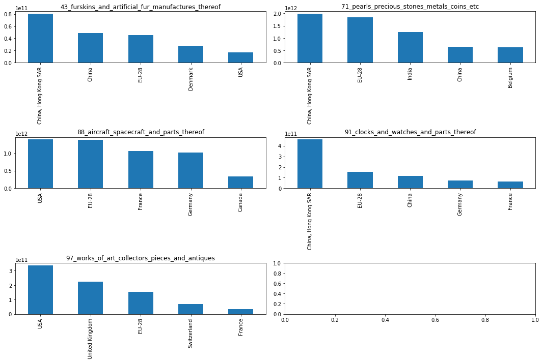
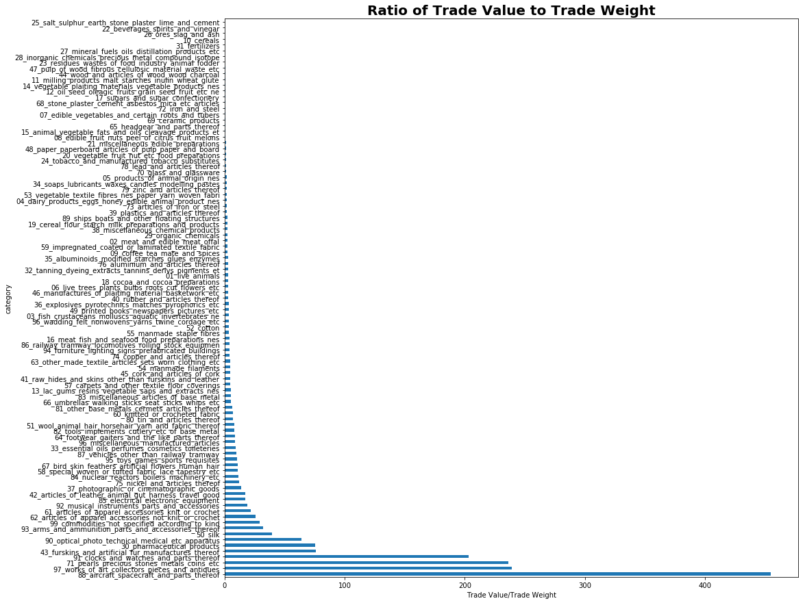
Now we can see where the value really lies, by taking the ratio of $\frac{Trade Value}{Trade Weight}$ we can get an idea of what has the highest value to weight ratio. Not unsurprisingly, we see aircraft/spacecraft parts right up the top, followed by art/antiques, precious stones/coins, clocks/watches, furs and then pharmaceuticals. Now let’s see which countries are producing these!
fig, ax = plt.subplots(1,1)
value_weight = (category_value/category_weight)
value_weight.sort_values(ascending=False).plot(kind='barh', figsize=(15,15))
plt.title('Ratio of Trade Value to Trade Weight', size=20, fontweight='bold')
fmt = '{x:,.0f}'
tick = mtick.StrMethodFormatter(fmt)
ax.xaxis.set_major_formatter(tick)
plt.xlabel('Trade Value/Trade Weight')
plt.show()
top_valueweight = value_weight.sort_values(ascending=False).index[0:5]
country_category = df.groupby(['country_or_area', 'category'])['trade_usd'].sum().unstack()
country_category = country_category.loc[:, country_category.columns.isin(top_valueweight)]
We see a common trend. USA, China and EU appear quite frequently in the trade of the highest value items. Note we haven’t split by import/exports here, just net involvement in the trade of said items.
fig, ax = plt.subplots(3, 2, figsize=(15,10))
for i, j in enumerate(country_category):
    country_category[j].sort_values(ascending=False).head(5).plot(kind='bar', title=j, ax=ax.flat[i])
    ax.flat[i].set_xlabel('')

plt.tight_layout()
plt.show()