Sentiment Analysis of Financial News Headlines Using NLP

Given the explosion of unstructured data through the growth in social media, there’s going to be more and more value attributable to insights we can derive from this data. One of particular interest is the application to finance. Many people (and corporations) seek to answer whether there is any exploitable relationships between this unstructured data and financial assets. Provided one could come up with a robust algorithm, there is likely significant scope for implementation.

Here we will look at some data provided by Kaggle, and see what we can learn through frequency analysis, TF-IDF analysis and the application of some basic prediction/regression.

Data here

import pandas as pd
import numpy as np
import matplotlib.pyplot as plt

from nltk.sentiment.vader import SentimentIntensityAnalyzer # VADER https://github.com/cjhutto/vaderSentiment
from nltk import tokenize

df = pd.read_csv("D:\Downloads\Data\stocknews\Combined_News_DJIA.csv")
dj_df = pd.read_csv("D:\Downloads\Data\stocknews\DJIA_table.csv")
reddit_df = pd.read_csv("D:\Downloads\Data\stocknews\RedditNews.csv")

df.describe()
df.Date = pd.to_datetime(df.Date)
df.head()
df.index = df.Date

dj_df.describe()
dj_df.Date = pd.to_datetime(dj_df.Date)
dj_df.index = dj_df.Date
dj_df = dj_df.sortb_values(by = 'Date', ascending=True)
dj_df.head()

	Date	Open	High	Low	Close	Volume	Adj Close
Date
2008-08-08	2008-08-08	11432.089844	11759.959961	11388.040039	11734.320312	212830000	11734.320312
2008-08-11	2008-08-11	11729.669922	11867.110352	11675.530273	11782.349609	183190000	11782.349609
2008-08-12	2008-08-12	11781.700195	11782.349609	11601.519531	11642.469727	173590000	11642.469727
2008-08-13	2008-08-13	11632.809570	11633.780273	11453.339844	11532.959961	182550000	11532.959961
2008-08-14	2008-08-14	11532.070312	11718.280273	11450.889648	11615.929688	159790000	11615.929688

reddit_df.index = pd.to_datetime(reddit_df.Date)

Frequency Analysis

from sklearn.feature_extraction.text import CountVectorizer
from sklearn.linear_model import LogisticRegression
from nltk.corpus import stopwords
stop = set(stopwords.words('english'))

# Create a single string for each date (since we only want to look at word counts)
news_combined = ''
for row in range(0,len(df.index)):
    news_combined+=' '.join(str(x).lower().strip() for x in df.iloc[row,2:27])
    
vectorizer = CountVectorizer()
news_vect = vectorizer.build_tokenizer()(news_combined)
word_counts = pd.DataFrame([[x,news_vect.count(x)] for x in set(news_vect)], columns = ['Word', 'Count'])

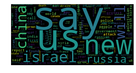
from wordcloud import WordCloud
wordcloud = WordCloud().generate(news_combined)
plt.imshow(wordcloud, interpolation='bilinear')
plt.axis("off")

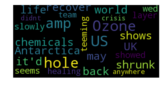
# lower max_font_size
wordcloud = WordCloud(max_font_size=40).generate(text)
plt.figure()
plt.imshow(wordcloud, interpolation="bilinear")
plt.axis("off")
plt.show()

png

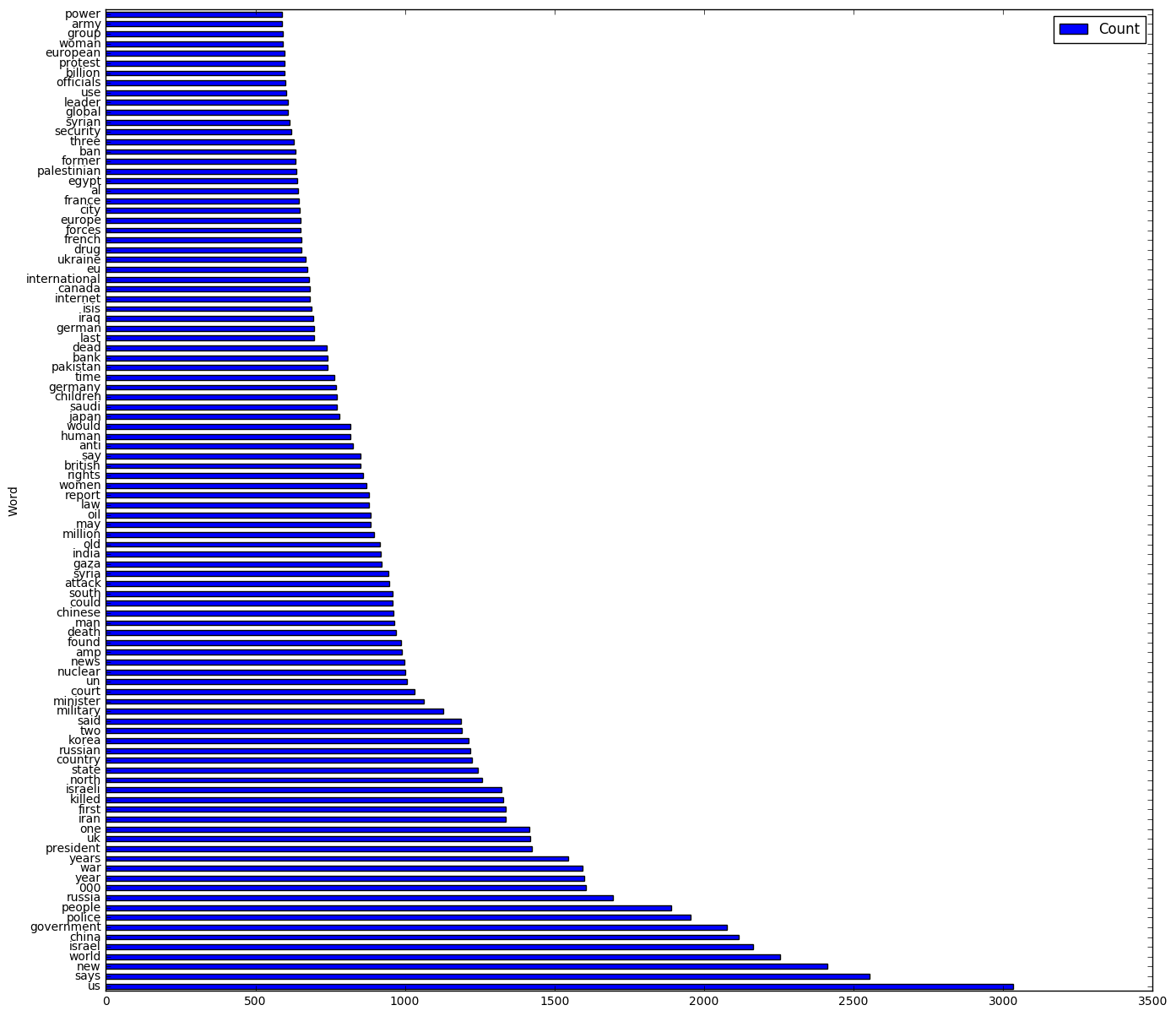
word_counts_adj = word_counts
word_counts_adj = word_counts_adj .reset_index(drop=True)

for i in word_counts['Word']:
    if i in stop:
        word_counts_adj = word_counts_adj.drop(word_counts_adj[word_counts_adj['Word'] == i].index)
        
word_counts_adj.index = word_counts_adj['Word']
counts = word_counts_adj.sort_values(by='Count', ascending=False)[0:100].plot(kind='barh', figsize = (16,15))
plt.show()

png

Sentiment Analysis

A large area of research is going into understanding unstructured data, and in particular seeing if we can harvest the constant streams of social media text coming from sources like Twitter, Reddit, News Headlines etc. Here we’ll have a look at some basic sentiment analysis and then see if we can attempt to classify changes in the S&P500 by looking at changes in the sentiment.

Financial News Headlines

The data provided consists of the top 25 headlines on Reddits r/worldnews each day from 2008-08-08 to 2016-07-01.

scores = pd.DataFrame(index = df.Date, columns = ['Compound', 'Positive', 'Negative', "Neutral"])

analyzer = SentimentIntensityAnalyzer() # Use the VADER Sentiment Analyzer

for j in range(1,df.shape[0]):    
    tmp_neu = 0
    tmp_neg = 0
    tmp_pos = 0
    tmp_comp = 0
    for i in range(2,df.shape[1]):
        text = df.iloc[j,i]
        if(str(text) == "nan"):
            tmp_comp +=  0
            tmp_neg += 0
            tmp_neu += 0
            tmp_pos += 0
        else:
            vs = analyzer.polarity_scores(df.iloc[j,i])
            tmp_comp +=  vs['compound']
            tmp_neg += vs['neg']
            tmp_neu += vs['neu']
            tmp_pos += vs['pos']
    
    scores.iloc[j,] = [tmp_comp, tmp_pos, tmp_neg, tmp_neu]

scores.head()
scores = scores.dropna()

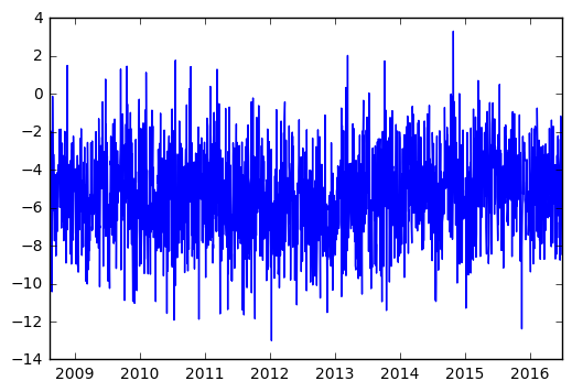
We can see that on average the news headlines in r/worldnews tend to be quite negative. This is not unexpected given the often political nature of the Subreddit, and corroborates with the frequency analysis showing words like ‘china’, ‘israel’, ‘government’, ‘war’, ‘nuclear’, ‘court’ are among the most frequently found words.

scores.index = scores.index.to_datetime()
plt.plot(scores.Compound)
plt.show()

png

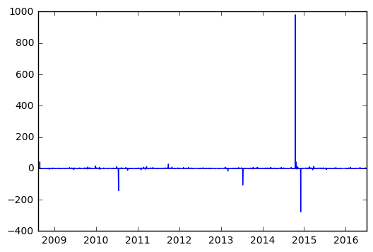
We can also start to see if there’s any relationship between movements in the Dow Jones Index and our sentiment scores. WE first notice that if we look at returns, there are some extreme outliers in the sentinment analysis. This is likely a product of basically a “0” sentinment being assigned to a day and blowing out any subsequent change. For now, we’ll simply work on a difference basis to see what we can draw out of the data.

plt.plot(scores.index, scores.Compound.shift(1)/scores.Compound-1)
plt.show()

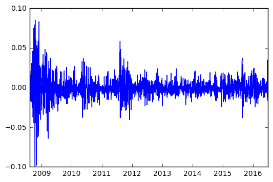
plt.plot(dj_df.Date, dj_df.Close.shift(1)/dj_df.Close-1)
plt.show()

plt.scatter(np.diff(dj_df.Close), np.diff(scores.Compound))
plt.show()

png

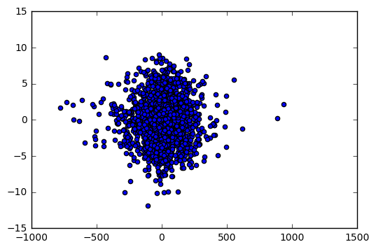
…and our answer is… not much. It doesn’t look like there’s any strong relationship between our sentinment changes and DJIA changes. This is not surprising, given that we’re using a very specific microcosm of the internet (Reddit r/worldnews) which likely contains biased information. Perhaps something more interesting we can explore is a time-series decomposition of the data.. but first we’ll implement some basic binary classifiers to see just how poor the relationship is.

# Import classifiers
from sklearn.neighbors import KNeighborsRegressor
from sklearn.svm import SVC
from sklearn.naive_bayes import GaussianNB
from sklearn.discriminant_analysis import LinearDiscriminantAnalysis
from sklearn.linear_model import  LinearRegression,  LogisticRegression

#Import helper functions
from sklearn.model_selection import learning_curve, train_test_split

import time

# Names of classifiers we want to use
clf_names = ["KNN",
             "Linear SVM",
             "RBF SVM",
             "Naive Bayes", 
             "LDA",
             "Linear Regression",
             "Logistic Regression",
            ]

# Implementation of each classifier we want to use, large scope in here for parameter tuning etc.
clfs = [KNeighborsRegressor(2),
        SVC(kernel="linear", C=0.025),
        SVC(gamma=2, C=1),
        GaussianNB(),
        LinearDiscriminantAnalysis(),
        LogisticRegression(), 

       ]

# Create test/train splits, and initialise plotting requirements
# We won't apply on feature reduction here, but it can be explored.
merged = scores.join(df)
merged = merged.iloc[:, 0:6]
merged = merged.iloc[2:,]
merged = merged.dropna()
train = merged[merged.index < '2015-01-01']
test = merged[merged.index > '2014-12-31']

#X_train, X_test, y_train, y_test = train_test_split(X, y, test_size=.33, random_state=42)
X_train = train[['Compound']]#.reshape(-1,1)
X_test = test[['Compound']]#.reshape(-1,1)
y_train = train['Label'].reshape(-1,1)
y_test = test['Label'].reshape(-1,1)

regressor_data = pd.DataFrame(columns = ["Name", "Score", "Training_Time"])
fig = plt.figure(figsize = (15,60))
i = 0

# Iterate over each regressor (no cross validation/KFolds yet)
for name, clf in zip(clf_names, clfs):
    print("#" * 80)
    print("Fitting '%s' regressor." % name)
    
    # Time required to fit the regressor
    t0 = time.time()
    clf.fit(X_train, y_train.ravel())
    t1 = time.time()

    score = clf.score(X_test, y_test.ravel())
    print("Name: %s Score: %.2f Time %.4f secs" % (name, score, t1-t0))
    
    # Store results
    regressor_data.loc[i] = [name, score, t1-t0]
    i += 1

################################################################################
Fitting 'KNN' regressor.
Name: KNN Score: -0.50 Time 0.0020 secs
################################################################################
Fitting 'Linear SVM' regressor.
Name: Linear SVM Score: 0.51 Time 0.0350 secs
################################################################################
Fitting 'RBF SVM' regressor.
Name: RBF SVM Score: 0.47 Time 0.1041 secs
################################################################################
Fitting 'Naive Bayes' regressor.
Name: Naive Bayes Score: 0.47 Time 0.0010 secs
################################################################################
Fitting 'LDA' regressor.
Name: LDA Score: 0.48 Time 0.0010 secs
################################################################################
Fitting 'Linear Regression' regressor.
Name: Linear Regression Score: 0.48 Time 0.0010 secs

As expected, we see scores in the order of 0.50.. i.e. we’re no better off flipping a coin than using the reddit r/worldnews to try and guess the direction of the market. Importantly, we note that we’ve used the sentiment on a day to classify whether the current day has gone up/down relative to the previous day. More accurately, we should look at the previous day’s headline and see if that can be used… since then we might gain an information advantage that we could exploit.

# Create test/train splits, and initialise plotting requirements
# We won't apply on feature reduction here, but it can be explored.
merged = scores.join(df)
merged = merged.iloc[:, 0:6]
merged = merged.iloc[2:,]
merged = merged.dropna()
train = merged[merged.index < '2015-01-01']
test = merged[merged.index > '2014-12-31']

# Here we adjust our train/test sets so that we're using the current days sentiment to predict tomorrow's change
X_train = train[['Compound']].shift(1)#.reshape(-1,1)
X_test = test[['Compound']].shift(1)#.reshape(-1,1)
X_train = X_train.dropna()
X_test = X_test.dropna()
y_train = train['Label'].reshape(-1,1)
y_train = y_train[:-1]
y_test = test['Label'].reshape(-1,1)
y_test = y_test[:-1]

regressor_data = pd.DataFrame(columns = ["Name", "Score", "Training_Time"])
fig = plt.figure(figsize = (15,60))
i = 0

# Iterate over each regressor (no cross validation/KFolds yet)
for name, clf in zip(clf_names, clfs):
    print("#" * 80)
    print("Fitting '%s' regressor." % name)
    
    # Time required to fit the regressor
    t0 = time.time()
    clf.fit(X_train, y_train.ravel())
    t1 = time.time()

    score = clf.score(X_test, y_test.ravel())
    print("Name: %s Score: %.2f Time %.4f secs" % (name, score, t1-t0))
    
    # Store results
    regressor_data.loc[i] = [name, score, t1-t0]
    i += 1

################################################################################
Fitting 'KNN' regressor.
Name: KNN Score: -0.49 Time 0.0020 secs
################################################################################
Fitting 'Linear SVM' regressor.
Name: Linear SVM Score: 0.51 Time 0.0240 secs
################################################################################
Fitting 'RBF SVM' regressor.
Name: RBF SVM Score: 0.47 Time 0.1041 secs
################################################################################
Fitting 'Naive Bayes' regressor.
Name: Naive Bayes Score: 0.48 Time 0.0010 secs
################################################################################
Fitting 'LDA' regressor.
Name: LDA Score: 0.48 Time 0.0020 secs
################################################################################
Fitting 'Linear Regression' regressor.
Name: Linear Regression Score: 0.48 Time 0.0010 secs

TF-IDF Analysis

An awesome tutorial here by Steven Loria gave me the idea of seeing if we can identify what were the key global trends in r/worldnews over the past few years. The tool being used here is TF-IDF (Term Frequency, Inverse Document Frequency) which is a way of scoring/ranking words by looking at their frequency both within a “document” and across other documents. Basically, it plays off between how frequency a word occurs in a document, and then the global “uniqueness” of that word across multiple documents. The more frequent, and more unique a word, the higher a score.

import math
from textblob import TextBlob as tb

def tf(word, blob):
    return blob.words.count(word) / len(blob.words)

def n_containing(word, bloblist):
    return sum(1 for blob in bloblist if word in blob.words)

def idf(word, bloblist):
    return math.log(len(bloblist) / (1 + n_containing(word, bloblist)))

def tfidf(word, blob, bloblist):
    return tf(word, blob) * idf(word, bloblist)

docs = pd.DataFrame(index=df.Date, columns=['Comb'])
for row in range(0,len(df.index)):
    docs.iloc[row,] = ' '.join(str(x).lower().strip().replace("b'", "").replace('b"', "") for x in df.iloc[row,2:27])
    

doc_2008 = docs[docs.index < "2009-01-01"].Comb.str.cat(sep = ' ').lower()
doc_2009 = docs[(docs.index >= "2009-11-01") & (docs.index < "2010-01-01")].Comb.str.cat(sep = ' ').lower()
doc_2010 = docs[(docs.index >= "2010-11-01") & (docs.index < "2011-01-01")].Comb.str.cat(sep = ' ').lower()
doc_2011 = docs[(docs.index >= "2011-11-01") & (docs.index < "2012-01-01")].Comb.str.cat(sep = ' ').lower()
doc_2012 = docs[(docs.index >= "2012-11-01") & (docs.index < "2013-01-01")].Comb.str.cat(sep = ' ').lower()
doc_2013 = docs[(docs.index >= "2013-11-01") & (docs.index < "2014-01-01")].Comb.str.cat(sep = ' ').lower()
doc_2014 = docs[(docs.index >= "2014-11-01") & (docs.index < "2015-01-01")].Comb.str.cat(sep = ' ').lower()
doc_2015 = docs[(docs.index >= "2015-11-01") & (docs.index < "2016-01-01")].Comb.str.cat(sep = ' ').lower()
doc_2016 =docs[(docs.index >= "2016-06-01") & (docs.index < "2017-01-01")].Comb.str.cat(sep = ' ').lower()

#bloblist = [tb(doc_2008), tb(doc_2009), tb(doc_2010), tb(doc_2011), tb(doc_2012), tb(doc_2013), tb(doc_2014)
#           , tb(doc_2015), tb(doc_2016)]

bloblist = [tb(doc_2008), tb(doc_2009), tb(doc_2010), tb(doc_2011), tb(doc_2012)
           , tb(doc_2013), tb(doc_2014), tb(doc_2015), tb(doc_2016)]

for i, blob in enumerate(bloblist):
    print("Top words in document year {}".format(i + 2008))
    scores = {word: tfidf(word, blob, bloblist) for word in (set(blob.words)-stop)}
    sorted_words = sorted(scores.items(), key=lambda x: x[1], reverse=True)
    for word, score in sorted_words[:5]:
        print("\tWord: {}, TF-IDF: {}".format(word, round(score, 5)))

Top words in document year 2008
	Word: georgia, TF-IDF: 0.00244
	Word: georgian, TF-IDF: 0.0013
	Word: ossetia, TF-IDF: 0.00102
	Word: mugabe, TF-IDF: 0.00036
	Word: hindu, TF-IDF: 0.00029
Top words in document year 2009
	Word: minarets, TF-IDF: 0.00054
	Word: copenhagen, TF-IDF: 0.00045
	Word: libel, TF-IDF: 0.00039
	Word: r\n, TF-IDF: 0.00039
	Word: swine, TF-IDF: 0.00039
Top words in document year 2010
	Word: cables, TF-IDF: 0.00133
	Word: assange, TF-IDF: 0.00109
	Word: manning, TF-IDF: 0.0007
	Word: mastercard, TF-IDF: 0.00063
	Word: julian, TF-IDF: 0.00056
Top words in document year 2011
	Word: hormuz, TF-IDF: 0.00052
	Word: strait, TF-IDF: 0.00045
	Word: eurozone, TF-IDF: 0.00044
	Word: tahrir, TF-IDF: 0.00043
	Word: homs, TF-IDF: 0.00038
Top words in document year 2012
	Word: morsi, TF-IDF: 0.00062
	Word: mayan, TF-IDF: 0.00054
	Word: mali, TF-IDF: 0.0004
	Word: non-member, TF-IDF: 0.00039
	Word: halappanavar, TF-IDF: 0.00031
Top words in document year 2013
	Word: nsa, TF-IDF: 0.00237
	Word: snowden, TF-IDF: 0.0018
	Word: edward, TF-IDF: 0.00108
	Word: pussy, TF-IDF: 0.00061
	Word: fukushima, TF-IDF: 0.00058
Top words in document year 2014
	Word: isis, TF-IDF: 0.0018
	Word: ruble, TF-IDF: 0.00117
	Word: sony, TF-IDF: 0.00098
	Word: airasia, TF-IDF: 0.0005
	Word: mistral, TF-IDF: 0.0005
Top words in document year 2015
	Word: isis, TF-IDF: 0.00373
	Word: ramadi, TF-IDF: 0.0005
	Word: tpp, TF-IDF: 0.00049
	Word: downed, TF-IDF: 0.00043
	Word: daesh, TF-IDF: 0.00042
Top words in document year 2016
	Word: brexit, TF-IDF: 0.00298
	Word: isis, TF-IDF: 0.0013
	Word: ramadan, TF-IDF: 0.00071
	Word: farage, TF-IDF: 0.00071
	Word: bookseller, TF-IDF: 0.00057

Some quite interesting results. Note that we’ve only looked at November & December in each year due to the increasing computational time when looking at an entire year of data. We see that some of the key events in that time are called out:

2009: Swiss-minaret referendum, Swine flu pandemic
2010: Julian Assange’s 2010 extradition request, US Cables Leak,
2016: Brexit, Nigel Farage

So we can see that this is a pretty interesting tool for highlighting from large sets of information, key topics and points of interest. This could have particular use in say deconstructing analyst equity reports across periods of time to pull out trends/thematic concerns.