Analysis of Key Fincial Indices, Sectors and Something Extra for Renewable Energy Stocks
I built out this as my own tool to track various things I’m interested in: indices, FX, rates, commodities and specific equities. It leverages various Quandl datasets, as well as my own database of equities data that I’ve accumulated from various sources (check here for set-up of DB).
import pandas as pd
import numpy as np
import matplotlib.pyplot as plt
import quandl

quandl.ApiConfig.api_key = "insert api key here"
Fundamentals Data
This gives me a snapshot of key metrics I’m interested in across various things (DJIA, FX, Bitcoin, Iron Ore etc) via some basis charts, and then some returns analysis. Most data is sourced from various free Quandl databases.
curr_date = pd.datetime(2017,6,17)
start_date = curr_date - pd.DateOffset(years=1)
save_path = "C:\\Users\\Clint_PC\\Google Drive\\General Learning\\Python\\Learning Plan Code\\Finance\\Results Tables\\"
#[SP500, SP500 VIX, DJIA_VIX, NASDAQ, DAX_future, FTSE100, Nikkei, Shanghai ]
index_quandlcodes = ['CHRIS/CME_SP1.4',
                     'CBOE/VIX.2',
                     'CBOE/VXD.2',
                     'NASDAQOMX/COMP.1',
                     'CHRIS/EUREX_FDAX1.2',
                     'CHRIS/LIFFE_Z1.2',
                     'NIKKEI/INDEX.4']
#[AUD, EUR, GBP, JPY]
fx_quandlcodes = ['FRED/DEXUSAL',
                 'FRED/DEXUSEU',
                 'FRED/DEXUSUK',
                 'FRED/DEXJPUS']

#[Ave Price, Num Transactions, Market Cap, Total Bitcoin]
bitcoin_quandlcodes = ['BCHARTS/BITSTAMPUSD.7',
                      'BCHAIN/NTRAN',
                      'BCHAIN/MKTCP',
                      'BCHAIN/TOTBC']
#[Crude, Gold, Iron Ore (NYMEX traded 62% Fe, CFR China in $US/metric tonne)]
commodities_quandlcodes = ['CHRIS/CME_CL1.4',
                          'LBMA/GOLD.2',
                          'COM/FE_TJN']

#[USD Long Term, USD10y, ON USDLibor, 1y USD T Bill]
rates_quandlcodes = ['USTREASURY/LONGTERMRATES.1',
                    'FRED/DGS10',
                    'FRED/DTB1YR']

#[CDX NA Inv. Grade, CDX NA High Yield]
credit_quandlcodes = ['COM/CDXNAIG',
                     'COM/CDXNAHY']
#aud_quandlcodes = ['RBA/H01.1',
#                  'RBA/G01.1']


all_codes = index_quandlcodes + fx_quandlcodes + bitcoin_quandlcodes + commodities_quandlcodes + rates_quandlcodes + credit_quandlcodes

equities = ['test', 'test2', 'test3']
renewable_energy_stocks = ['test4', 'test5', 'test6']
all_codes
['CHRIS/CME_SP1.4',
 'CBOE/VIX.2',
 'CBOE/VXD.2',
 'NASDAQOMX/COMP.1',
 'CHRIS/EUREX_FDAX1.2',
 'CHRIS/LIFFE_Z1.2',
 'NIKKEI/INDEX.4',
 'FRED/DEXUSAL',
 'FRED/DEXUSEU',
 'FRED/DEXUSUK',
 'FRED/DEXJPUS',
 'BCHARTS/BITSTAMPUSD.7',
 'BCHAIN/NTRAN',
 'BCHAIN/MKTCP',
 'BCHAIN/TOTBC',
 'CHRIS/CME_CL1.4',
 'LBMA/GOLD.2',
 'COM/FE_TJN',
 'USTREASURY/LONGTERMRATES.1',
 'FRED/DGS10',
 'FRED/DTB1YR',
 'COM/CDXNAIG',
 'COM/CDXNAHY']
vals = quandl.get(all_codes, start_date=start_date, end_date = curr_date)
Click to expand
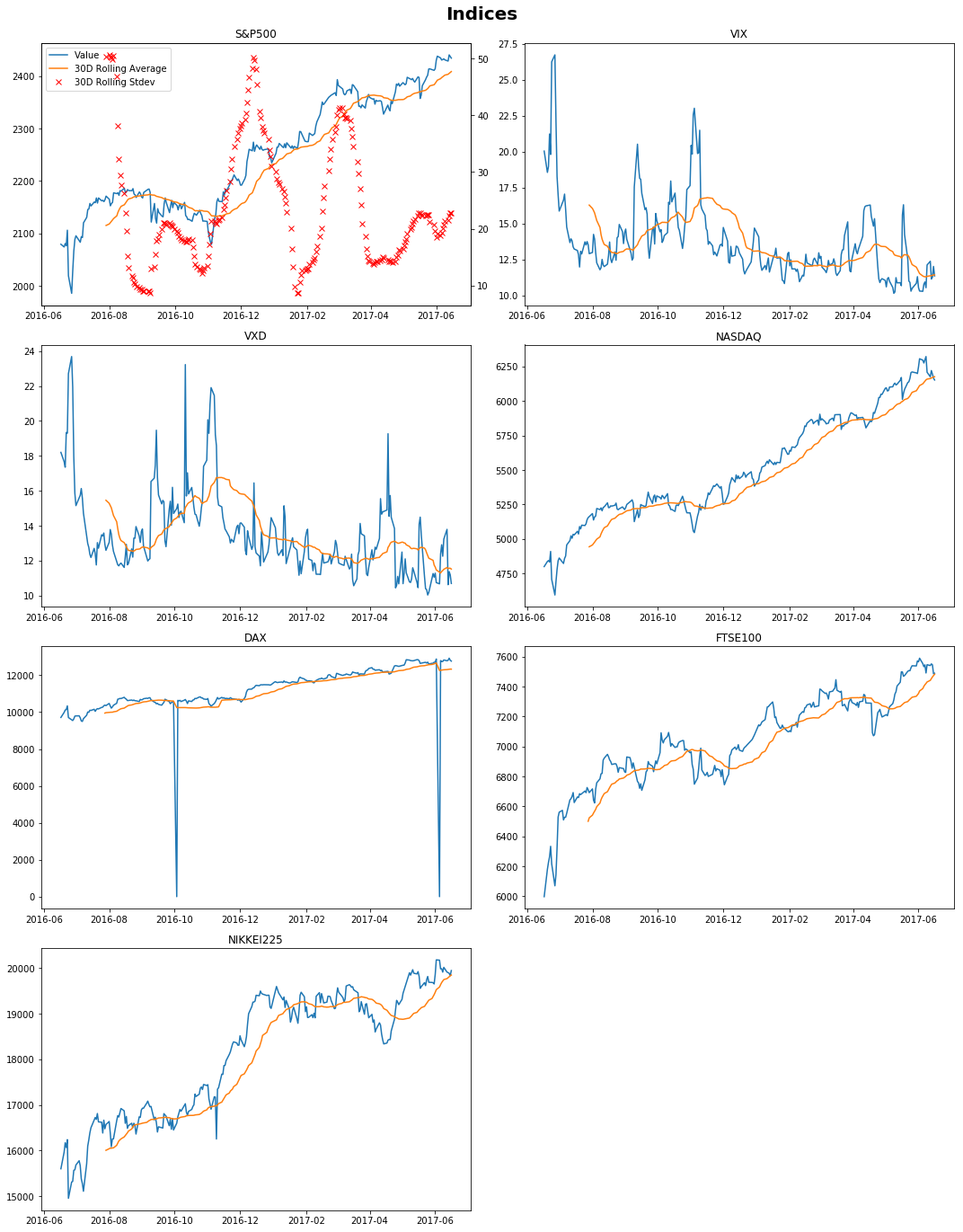
```python fig, ax = plt.subplots(nrows=4, ncols=2, sharex=False, sharey=False, figsize = (15,20)) fig.suptitle('Indices', fontsize=20, fontweight='bold') ax1 = plt.subplot(421) line1 = plt.plot(vals.iloc[:,0].dropna(), label = 'Value') line2 = plt.plot(vals.iloc[:,0].dropna().rolling(30).mean(), label = '30D Rolling Average') ax2 = ax1.twinx() line3 = ax2.plot(vals.iloc[:,0].dropna().rolling(30).std(), 'xr', label = '30D Rolling Stdev') ax2.yaxis.tick_right() ax2.yaxis.set_label_position("right") lns = line1+line2+line3 labs = [l.get_label() for l in lns] ax1.legend(lns, labs, loc=0) plt.title('S&P500') plt.subplot(4,2,2) plt.plot(vals.iloc[:,1].dropna()) plt.plot(vals.iloc[:,1].dropna().rolling(30).mean()) plt.title('VIX') plt.subplot(4,2,3) plt.plot(vals.iloc[:,2].dropna()) plt.plot(vals.iloc[:,2].dropna().rolling(30).mean()) plt.title('VXD') plt.subplot(4,2,4) plt.plot(vals.iloc[:,3].dropna()) plt.plot(vals.iloc[:,3].dropna().rolling(30).mean()) plt.title('NASDAQ') plt.subplot(4,2,5) plt.plot(vals.iloc[:,4].dropna()) plt.plot(vals.iloc[:,4].dropna().rolling(30).mean()) plt.title('DAX') plt.subplot(4,2,6) plt.plot(vals.iloc[:,5].dropna()) plt.plot(vals.iloc[:,5].dropna().rolling(30).mean()) plt.title('FTSE100') plt.subplot(4,2,7) plt.plot(vals.iloc[:,6].dropna()) plt.plot(vals.iloc[:,6].dropna().rolling(30).mean()) plt.title('NIKKEI225') fig.delaxes(ax.flatten()[7]) plt.tight_layout(rect=[0, 0.03, 1, 0.97]) plt.show() ```
Click to expand
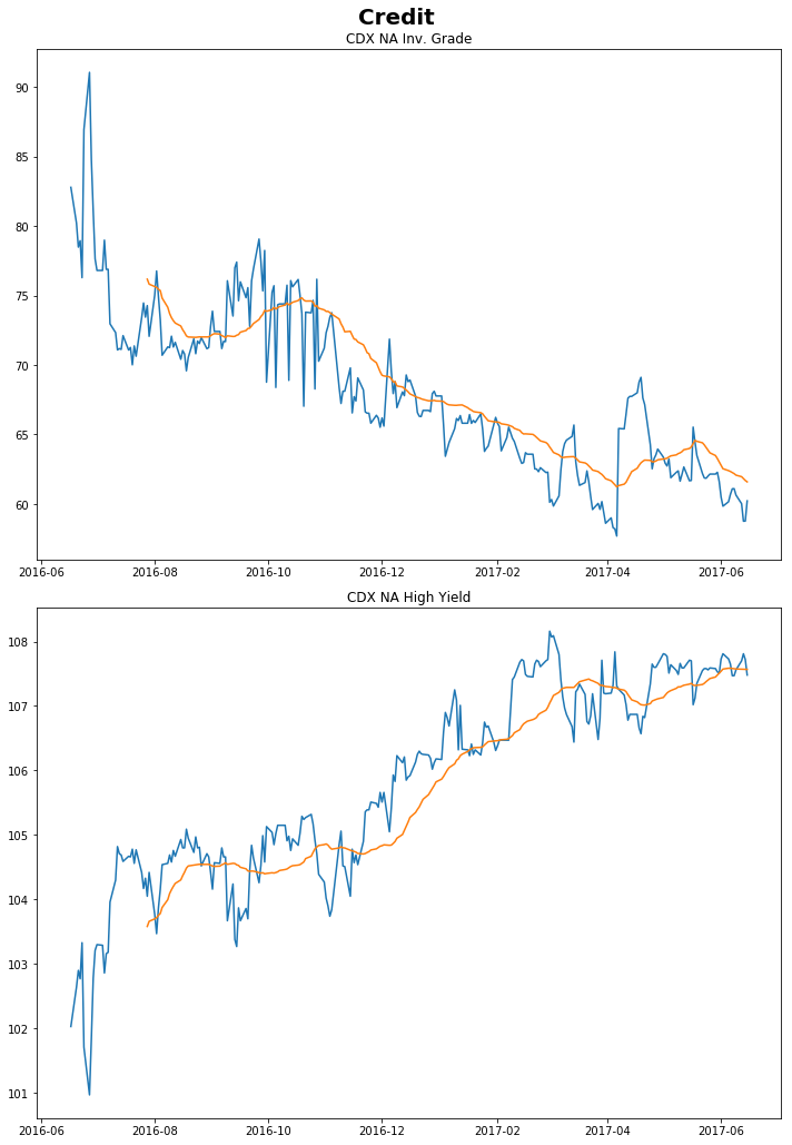
```python fig, ax = plt.subplots(nrows=2, ncols=1, sharex=True, sharey=False, figsize = (10,15)) fig.suptitle('Credit', fontsize=20, fontweight='bold') plt.subplot(211) plt.plot(vals.iloc[:,21].dropna()) plt.plot(vals.iloc[:,21].dropna().rolling(30).mean()) plt.title('CDX NA Inv. Grade') plt.subplot(212) plt.plot(vals.iloc[:,22].dropna()) plt.plot(vals.iloc[:,22].dropna().rolling(30).mean()) plt.title('CDX NA High Yield') plt.tight_layout(rect=[0, 0.03, 1, 0.97]) plt.show() ```
Click to expand
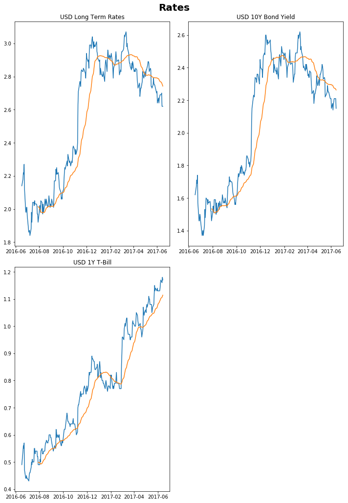
```python fig, ax = plt.subplots(nrows=2, ncols=2, sharex=True, sharey=False, figsize = (10,15)) fig.suptitle('Rates', fontsize=20, fontweight='bold') plt.subplot(2,2,1) plt.plot(vals.iloc[:,18].dropna()) plt.plot(vals.iloc[:,18].dropna().rolling(30).mean()) plt.title('USD Long Term Rates') plt.subplot(2,2,2) plt.plot(vals.iloc[:,19].dropna()) plt.plot(vals.iloc[:,19].dropna().rolling(30).mean()) plt.title('USD 10Y Bond Yield') plt.subplot(2,2,3) plt.plot(vals.iloc[:,20].dropna()) plt.plot(vals.iloc[:,20].dropna().rolling(30).mean()) plt.title('USD 1Y T-Bill') fig.delaxes(ax.flatten()[3]) plt.tight_layout(rect=[0, 0.03, 1, 0.97]) plt.show() ```
Click to expand
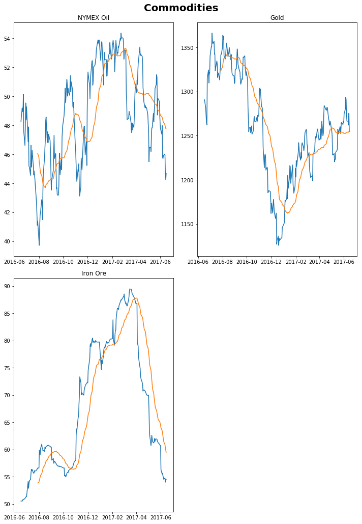
```python fig, ax = plt.subplots(nrows=2, ncols=2, sharex=True, sharey=False, figsize = (10,15)) fig.suptitle('Commodities', fontsize=20, fontweight='bold') plt.subplot(2,2,1) plt.plot(vals.iloc[:,15].dropna()) plt.plot(vals.iloc[:,15].dropna().rolling(30).mean()) plt.title('NYMEX Oil') plt.subplot(2,2,2) plt.plot(vals.iloc[:,16].dropna()) plt.plot(vals.iloc[:,16].dropna().rolling(30).mean()) plt.title('Gold') plt.subplot(2,2,3) plt.plot(vals.iloc[:,17].dropna()) plt.plot(vals.iloc[:,17].dropna().rolling(30).mean()) plt.title('Iron Ore') fig.delaxes(ax.flatten()[3]) plt.tight_layout(rect=[0, 0.03, 1, 0.97]) plt.show() ```
Click to expand
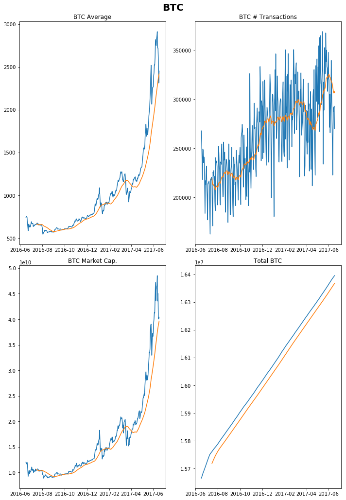
```python fig, ax = plt.subplots(nrows=2, ncols=2, sharex=True, sharey=False, figsize = (10,15)) fig.suptitle('BTC', fontsize=20, fontweight='bold') plt.subplot(2,2,1) plt.plot(vals.iloc[:,11].dropna()) plt.plot(vals.iloc[:,11].dropna().rolling(30).mean()) plt.title('BTC Average') plt.subplot(2,2,2) plt.plot(vals.iloc[:,12].dropna()) plt.plot(vals.iloc[:,12].dropna().rolling(30).mean()) plt.title('BTC # Transactions') plt.subplot(2,2,3) plt.plot(vals.iloc[:,13].dropna()) plt.plot(vals.iloc[:,13].dropna().rolling(30).mean()) plt.title('BTC Market Cap.') plt.subplot(2,2,4) plt.plot(vals.iloc[:,14].dropna()) plt.plot(vals.iloc[:,14].dropna().rolling(30).mean()) plt.title('Total BTC') plt.tight_layout(rect=[0, 0.03, 1, 0.97]) plt.show() ```
Click to expand
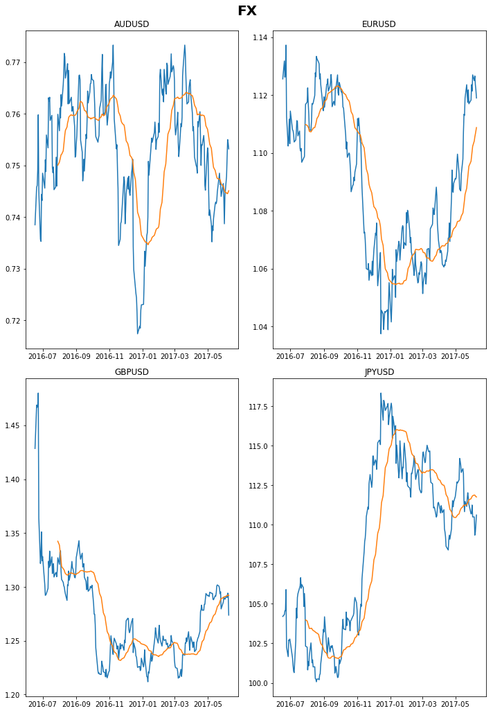
```python fig, ax = plt.subplots(nrows=2, ncols=2, sharex=True, sharey=True, figsize = (10,15)) fig.suptitle('FX', fontsize=20, fontweight='bold') plt.subplot(2,2,1) plt.plot(vals.iloc[:,7].dropna()) plt.plot(vals.iloc[:,7].dropna().rolling(30).mean()) plt.title('AUDUSD') plt.subplot(2,2,2) plt.plot(vals.iloc[:,8].dropna()) plt.plot(vals.iloc[:,8].dropna().rolling(30).mean()) plt.title('EURUSD') plt.subplot(2,2,3) plt.plot(vals.iloc[:,9].dropna()) plt.plot(vals.iloc[:,9].dropna().rolling(30).mean()) plt.title('GBPUSD') plt.subplot(2,2,4) plt.plot(vals.iloc[:,10].dropna()) plt.plot(vals.iloc[:,10].dropna().rolling(30).mean()) plt.title('JPYUSD') plt.tight_layout(rect=[0, 0.03, 1, 0.97]) plt.show() fig.savefig(save_path+"FX_"+str(curr_date)[0:10]) ```
results = pd.DataFrame(index=vals.columns, columns = ['Description','Data_Date','Spot', 'Daily', 'WTD', 'MTD', 'YTD', 'YoY'])
results['Description'] = ['S&P500 Futures',
                         'S&P500 VIX',
                         'DJIA VXD',
                         'NASDAQ',
                         'DAX',
                         'FTSE100',
                         'NIKKEI225',
                         'AUDUSD',
                         'EURUSD',
                         'GBPUSD',
                         'JPYUSD',
                         'Average BTC Price',
                         'BTC # Transactions',
                         'BTC Market Cap.',
                         'Total BTC',
                         'NYMEX Crude Oil',
                         'Gold',
                         'Iron Ore 62%',
                         'USD Long Term Rate',
                         'USD 10Y Bond Yield',
                         'USD 1Y T-Bill',
                         'CDX NA Investment Grade',
                         'CDX NA High Yield']

for col in vals.columns:
    prices = vals[col]
    prices = prices.dropna()

    last_date = prices.last_valid_index()
    prior_date = last_date - pd.tseries.offsets.Day(days=1)

    start = prices.index[0]

    week = last_date - pd.tseries.offsets.Week(weekday=0)
    week = prices.index.get_loc(week,method='nearest')

    month = last_date - pd.tseries.offsets.BMonthBegin()
    month = prices.index.get_loc(month,method='nearest')

    year = last_date - pd.tseries.offsets.BYearBegin()
    year = prices.index.get_loc(year,method='nearest')

    close = prices[last_date]
    daily = round((close - prices[prior_date])/prices[prior_date]*100, 3)
    wtd = round((close - prices[week])/prices[week]*100, 3)
    mtd = round((close - prices[month])/prices[month]*100, 3)
    ytd = round((close - prices[year])/prices[year]*100, 3)
    yoy = round((close-prices[start])/prices[start]*100, 3)

    results.loc[col, ['Data_Date', 'Spot', 'Daily', 'WTD', 'MTD', 'YTD', 'YoY']] = [last_date, close, daily, wtd, mtd, ytd, yoy ]
results
| Description | Data_Date | Spot | Daily | WTD | MTD | YTD | YoY | |
|---|---|---|---|---|---|---|---|---|
| CHRIS/CME_SP1 - Last | S&P500 Futures | 2017-06-15 00:00:00 | 2434.3 | -0.123 | 0.231 | 0.177 | 8.061 | 17.083 |
| CBOE/VIX - VIX High | S&P500 VIX | 2017-06-16 00:00:00 | 11.35 | -5.495 | -8.246 | 7.685 | -19.332 | -43.335 |
| CBOE/VXD - High | DJIA VXD | 2017-06-16 00:00:00 | 10.69 | -4.383 | -22.48 | -5.23 | -22.983 | -41.264 |
| NASDAQOMX/COMP - Index Value | NASDAQ | 2017-06-16 00:00:00 | 6151.76 | -0.223 | -0.384 | -1.522 | 13.311 | 28.153 |
| CHRIS/EUREX_FDAX1 - High | DAX | 2017-06-16 00:00:00 | 12765 | -0.375 | -0.153 | 0.54 | 9.83 | 31.429 |
| CHRIS/LIFFE_Z1 - High | FTSE100 | 2017-06-16 00:00:00 | 7489 | 0.053 | -0.676 | -1.005 | 4.829 | 24.858 |
| NIKKEI/INDEX - Close Price | NIKKEI225 | 2017-06-16 00:00:00 | 19943.3 | 0.562 | 0.174 | 0.419 | 1.782 | 27.844 |
| FRED/DEXUSAL - Value | AUDUSD | 2017-06-09 00:00:00 | 0.7532 | -0.146 | 0.709 | 1.963 | 4.163 | 1.991 |
| FRED/DEXUSEU - Value | EURUSD | 2017-06-09 00:00:00 | 1.119 | -0.241 | -0.533 | -0.214 | 7.431 | -0.586 |
| FRED/DEXUSUK - Value | GBPUSD | 2017-06-09 00:00:00 | 1.2737 | -1.561 | -1.394 | -1.218 | 3.925 | -10.837 |
| FRED/DEXJPUS - Value | JPYUSD | 2017-06-09 00:00:00 | 110.61 | 0.463 | 0.109 | -0.566 | -6.008 | 6.152 |
| BCHARTS/BITSTAMPUSD - Weighted Price | Average BTC Price | 2017-06-16 00:00:00 | 2450.92 | 6.028 | -9.918 | 2.524 | 141.946 | 231.684 |
| BCHAIN/NTRAN - Value | BTC # Transactions | 2017-06-17 00:00:00 | 269937 | -7.916 | 21.107 | -16.073 | 49.548 | 0.772 |
| BCHAIN/MKTCP - Value | BTC Market Cap. | 2017-06-17 00:00:00 | 4.04131e+10 | 0.932 | -16.729 | 8.036 | 150.315 | 235.993 |
| BCHAIN/TOTBC - Value | Total BTC | 2017-06-17 00:00:00 | 1.6395e+07 | 0.011 | 0.056 | 0.19 | 1.976 | 4.656 |
| CHRIS/CME_CL1 - Last | NYMEX Crude Oil | 2017-06-16 00:00:00 | 44.68 | 0.995 | -2.87 | -6.975 | -14.847 | -7.418 |
| LBMA/GOLD - USD (PM) | Gold | 2017-06-16 00:00:00 | 1255.4 | 0.068 | -0.869 | -0.747 | 9.07 | -2.735 |
| COM/FE_TJN - Column 1 | Iron Ore 62% | 2017-06-15 00:00:00 | 54.51 | 0.018 | -0.475 | -10.212 | -26.989 | 7.834 |
| USTREASURY/LONGTERMRATES - LT Composite > 10 Yrs | USD Long Term Rate | 2017-06-16 00:00:00 | 2.62 | 0 | -2.602 | -3.321 | -9.343 | 22.43 |
| FRED/DGS10 - Value | USD 10Y Bond Yield | 2017-06-14 00:00:00 | 2.15 | -2.715 | -2.715 | -2.715 | -12.245 | 32.716 |
| FRED/DTB1YR - Value | USD 1Y T-Bill | 2017-06-14 00:00:00 | 1.17 | -0.847 | 0.862 | 3.54 | 34.483 | 138.776 |
| COM/CDXNAIG - value | CDX NA Investment Grade | 2017-06-15 00:00:00 | 60.22 | 2.467 | 0.333 | -0.446 | -11.141 | -27.253 |
| COM/CDXNAHY - value | CDX NA High Yield | 2017-06-15 00:00:00 | 107.48 | -0.223 | -0.204 | -0.232 | 1.234 | 5.342 |
pathres_to_save = save_path + str(curr_date)[0:10] + "_agg.csv"
pathdata_to_save = save_path + str(curr_date)[0:10] + "_data.csv"
results.to_csv(pathres_to_save)
vals.to_csv(pathdata_to_save)
Sector Trends
This section deals with some equities analysis. I leverage off my databse of equities to perform some high level sector analysis, this gives me a quick overview of what various industries have been doing relative to each other and I can then deep-dive into anything that piques my interest.
import pymysql
from sqlalchemy import create_engine
import pandas as pd
import matplotlib.pyplot as plt
import pandas.io.sql as psql

db_host = 'localhost'
db_user = 'username'
db_pass = 'password'
db_name = 'pricing'

con = pymysql.connect(db_host, db_user, db_pass, db_name)

sql_usd = """SELECT *
         FROM symbol AS sym
         INNER JOIN daily_price AS dp
         ON dp.symbol_id = sym.id
         where price_date > '2016-01-01' AND currency = 'USD'
         ORDER BY dp.price_date ASC
         ;"""

sql_aud = """SELECT *
         FROM symbol AS sym
         INNER JOIN daily_price AS dp
         ON dp.symbol_id = sym.id
         where price_date > '2016-01-01' AND currency = 'AUD'
         ORDER BY dp.price_date ASC
         ;"""

engine = create_engine('mysql+pymysql://username:password@localhost:3306/pricing')

# Create a pandas dataframe from the SQL query
with engine.connect() as conn, conn.begin():
    p_usd_data = pd.read_sql(sql_usd, con)
    p_aud_data = pd.read_sql(sql_aud, con)
AUD Sectors
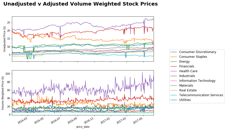
Here I leverage my AUD dataset to look at stock prices. I adjust based on volume… I would have preferred to have done it by Market Cap but haven’t got around to incorporating that into my scraper yet.
p_aud_data['volume_traded'] = p_aud_data.adj_close_price*p_aud_data.volume
total_marketcap = p_aud_data.groupby(['price_date', 'sector'])['volume_traded'].sum()
total_marketcap = total_marketcap.reset_index()
total_marketcap.columns = ['price_date', 'sector', 'total_volume_traded']
merged_aud_data = p_aud_data.merge(total_marketcap)
merged_aud_data['weighted_price'] =  merged_aud_data['adj_close_price']*merged_aud_data['volume_traded']/merged_aud_data['total_volume_traded']
fig, ax = plt.subplots(nrows=2, ncols=1, sharex=True, sharey=False, figsize = (10,8))
fig.suptitle('Unadjusted v Adjusted Volume Weighted Stock Prices', fontsize=20, fontweight='bold')

unadj_sectprices = p_aud_data.groupby(['price_date', 'sector'])['adj_close_price'].mean()
unadj_sectprices = unadj_sectprices.unstack()
unadj_sectprices.plot(ax=ax[0], legend = False)
ax[0].set_ylabel('Unadjusted Price ($)')

adj_sectorprices = merged_aud_data.groupby(['price_date', 'sector'])['weighted_price'].sum()
adj_sectorprices= adj_sectorprices.unstack()
adj_sectorprices = adj_sectorprices.dropna()

adj_sectorprices.plot(ax=ax[1])
ax[1].set_ylabel('Volume Weighted Price ($)')
plt.legend(bbox_to_anchor=(1.1, 1.5), prop={'size':12})
plt.show()
results_audsectors = pd.DataFrame(index=unadj_sectprices.columns, columns = ['Data_Date','Spot', 'Daily', 'WTD', 'MTD', 'YTD', 'YoY'])


for col in unadj_sectprices.columns:
    prices = unadj_sectprices[col]
    prices = prices.dropna()

    last_date = prices.last_valid_index()
    prior_date = last_date - pd.tseries.offsets.Day(days=2)

    start = prices.index[0]

    week = last_date - pd.tseries.offsets.Week(weekday=0)
    week = prices.index.get_loc(week,method='nearest')

    month = last_date - pd.tseries.offsets.BMonthBegin()
    month = prices.index.get_loc(month,method='nearest')

    year = last_date - pd.tseries.offsets.BYearBegin()
    year = prices.index.get_loc(year,method='nearest')

    close = prices[last_date]
    daily = round((close - prices[prior_date])/prices[prior_date]*100, 3)
    wtd = round((close - prices[week])/prices[week]*100, 3)
    mtd = round((close - prices[month])/prices[month]*100, 3)
    ytd = round((close - prices[year])/prices[year]*100, 3)
    yoy = round((close-prices[start])/prices[start]*100, 3)

    results_audsectors.loc[col, ['Data_Date', 'Spot', 'Daily', 'WTD', 'MTD', 'YTD', 'YoY']] = [last_date, close, daily, wtd, mtd, ytd, yoy ]
results_audsectors
| Data_Date | Spot | Daily | WTD | MTD | YTD | YoY | |
|---|---|---|---|---|---|---|---|
| sector | |||||||
| Consumer Discretionary | 2017-06-09 00:00:00 | 11.2737 | -0.144 | -5.988 | -1.477 | 3.026 | 15.742 |
| Consumer Staples | 2017-06-09 00:00:00 | 13.2524 | -0.561 | 18.072 | -5.876 | -2.883 | -32.342 |
| Energy | 2017-06-09 00:00:00 | 11.8119 | -1.568 | -5.164 | -4.309 | 3.019 | 11.897 |
| Financials | 2017-06-09 00:00:00 | 21.5229 | -0.089 | 10.438 | -0.899 | 1.907 | 6.242 |
| Health Care | 2017-06-09 00:00:00 | 26.9329 | -0.107 | -1.552 | 0.267 | 22.376 | 25.649 |
| Industrials | 2017-06-09 00:00:00 | 8.96132 | 0.283 | -8.559 | -0.812 | 13.241 | 35.912 |
| Information Technology | 2017-06-09 00:00:00 | 7.3155 | -0.184 | -2.408 | -0.469 | 1.463 | 15.954 |
| Materials | 2017-06-09 00:00:00 | 9.33486 | 0.891 | 3.22 | 0.913 | 2.208 | 45.456 |
| Real Estate | 2017-06-09 00:00:00 | 6.50386 | -0.369 | -3.879 | -3.604 | 2.136 | 55.885 |
| Telecommunication Services | 2017-06-09 00:00:00 | 4.3025 | 0.702 | 6.147 | 3.55 | -9.563 | -29.031 |
| Utilities | 2017-06-09 00:00:00 | 7.982 | 0.365 | -2.978 | -5.292 | 24.915 | 56.627 |
results_adjaudsectors = pd.DataFrame(index=adj_sectorprices.columns, columns = ['Data_Date','Spot', 'Daily', 'WTD', 'MTD', 'YTD', 'YoY'])

for col in adj_sectorprices.columns:
    prices = adj_sectorprices[col]
    prices = prices.dropna()

    last_date = prices.last_valid_index()
    prior_date = last_date - pd.tseries.offsets.Day(days=2)

    start = prices.index[0]

    week = last_date - pd.tseries.offsets.Week(weekday=0)
    week = prices.index.get_loc(week,method='nearest')

    month = last_date - pd.tseries.offsets.BMonthBegin()
    month = prices.index.get_loc(month,method='nearest')

    year = last_date - pd.tseries.offsets.BYearBegin()
    year = prices.index.get_loc(year,method='nearest')

    close = prices[last_date]
    daily = round((close - prices[prior_date])/prices[prior_date]*100, 3)
    wtd = round((close - prices[week])/prices[week]*100, 3)
    mtd = round((close - prices[month])/prices[month]*100, 3)
    ytd = round((close - prices[year])/prices[year]*100, 3)
    yoy = round((close-prices[start])/prices[start]*100, 3)

    results_adjaudsectors.loc[col, ['Data_Date', 'Spot', 'Daily', 'WTD', 'MTD', 'YTD', 'YoY']] = [last_date, close, daily, wtd, mtd, ytd, yoy ]
results_adjaudsectors
| Data_Date | Spot | Daily | WTD | MTD | YTD | YoY | |
|---|---|---|---|---|---|---|---|
| sector | |||||||
| Consumer Discretionary | 2017-06-09 00:00:00 | 17.4852 | -13.385 | -0.893 | -10.008 | 13.229 | 3.063 |
| Consumer Staples | 2017-06-09 00:00:00 | 25.0601 | 6.979 | 92.76 | -18.096 | -7.165 | 9.286 |
| Energy | 2017-06-09 00:00:00 | 17.3026 | -3.792 | -4.748 | -3.941 | 29.104 | -4.311 |
| Financials | 2017-06-09 00:00:00 | 38.5179 | 6.569 | -0.214 | 6.104 | -0.031 | 7.166 |
| Health Care | 2017-06-09 00:00:00 | 84.7876 | -8.615 | 1.844 | -1.168 | 49.879 | 55.14 |
| Industrials | 2017-06-09 00:00:00 | 8.70551 | -5.145 | -13.527 | -9.584 | -8.031 | 5.921 |
| Information Technology | 2017-06-09 00:00:00 | 8.70933 | -1.757 | -2.608 | -8.475 | 2.295 | 3.455 |
| Materials | 2017-06-09 00:00:00 | 17.466 | 8.354 | -5.28 | 1.476 | 5.38 | 26.412 |
| Real Estate | 2017-06-09 00:00:00 | 6.55767 | 1.143 | -0.893 | 3.349 | -1.541 | 21.346 |
| Telecommunication Services | 2017-06-09 00:00:00 | 4.28168 | 1.674 | 1.294 | -2.579 | -15.936 | -24.512 |
| Utilities | 2017-06-09 00:00:00 | 16.2257 | -2.395 | -4.747 | 11.369 | 56.829 | 73.865 |
USD Sectors
p_usd_data['volume_traded'] = p_usd_data.adj_close_price*p_usd_data.volume
total_marketcap = p_usd_data.groupby(['price_date', 'sector'])['volume_traded'].sum()
total_marketcap = total_marketcap.reset_index()
total_marketcap.columns = ['price_date', 'sector', 'total_volume_traded']
merged_usd_data = p_usd_data.merge(total_marketcap)
merged_usd_data['weighted_price'] =  merged_usd_data['adj_close_price']*merged_usd_data['volume_traded']/merged_usd_data['total_volume_traded']
fig, ax = plt.subplots(nrows=2, ncols=1, sharex=True, sharey=False, figsize = (10,8))
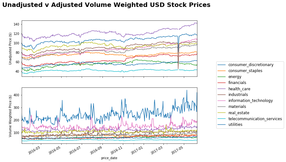
fig.suptitle('Unadjusted v Adjusted Volume Weighted USD Stock Prices', fontsize=20, fontweight='bold')
unadj_sectprices = p_usd_data.groupby(['price_date', 'sector'])['adj_close_price'].mean()
unadj_sectprices = unadj_sectprices.unstack()
unadj_sectprices.plot(ax=ax[0], legend = False)
ax[0].set_ylabel('Unadjusted Price ($)')
adj_sectorprices = merged_usd_data.groupby(['price_date', 'sector'])['weighted_price'].sum()
adj_sectorprices= adj_sectorprices.unstack()
adj_sectorprices = adj_sectorprices.dropna()
adj_sectorprices.plot(ax=ax[1])
ax[1].set_ylabel('Volume Weighted Price ($)')
plt.legend(bbox_to_anchor=(1.1, 1.5), prop={'size':12})
plt.show()
sectors = p_usd_data.groupby(['sector', 'subsector']).count()
sectors.reset_index(inplace=True)
np.unique(sectors[sectors.sector=='information_technology']['subsector'])
np.unique(sectors[sectors.sector=='financials']['subsector'])
array(['asset_management_&_custody_banks', 'consumer_finance',
       'diversified_banks', 'financial_exchanges_&_data',
       'insurance_brokers', 'investment_banking_&_brokerage',
       'life_&_health_insurance', 'multi-line_insurance',
       'multi-sector_holdings', 'property_&_casualty_insurance',
       'regional_banks', 'thrifts_&_mortgage_finance'], dtype=object)
Renewable Energy Stocks
Here I run some analysis on a renewable energy stocks. I first parse some in from Wikipedia, and then use an adapted Yahoo-API to pull in all the relevant data. Note that the Yahoo-API has been officially discontinued as at May-2017, so this process likely won’t last for long.
import datetime
from bs4 import BeautifulSoup
import urllib
import io
import requests
from math import ceil

# Function to pull table from Wikipedia containing Renewable Energy Companies
def obtain_parse_wiki_renewables():
    now = datetime.datetime.utcnow()
    url = "https://en.wikipedia.org/wiki/List_of_renewable_energy_companies_by_stock_exchange"
    request = urllib.request.Request(url)
    page = urllib.request.urlopen(request)
    soup = BeautifulSoup(page)

    table = soup.find("table", {"class": "wikitable sortable"})

    symbols = pd.DataFrame(columns=["Company", "Exchange", "Exchange_Ticker", "Stock_Ticker", "IPO_Date", "Industry"])

    for row in table.findAll("tr"):
        col = row.findAll("td")
        if len(col) > 0:
            try:
                company = str(col[0].find("a").string.strip()).lower().replace(" ", "_")
                exchange = str(col[1].find("a").string.strip()).lower().replace(" ", "_")
                exc_ticker = str(col[2].findAll("a")[0].string.strip())
                stock_ticker = str(col[2].findAll("a")[1].string.strip())
                if(len(col[3]) == 0):
                    ipo_date = "-"
                else:
                    ipo_date = str(col[3].string.strip())
                industry = str(col[4].string.strip().lower().replace(" ", "_"))

                symbols.loc[len(symbols)] = [company, exchange, exc_ticker, stock_ticker, ipo_date, industry]
            except:
                print("Passed.")

    return symbols

symbols1 = obtain_parse_wiki_renewables()
C:\Users\Clint_PC\Anaconda3\lib\site-packages\bs4\__init__.py:181: UserWarning: No parser was explicitly specified, so I'm using the best available HTML parser for this system ("lxml"). This usually isn't a problem, but if you run this code on another system, or in a different virtual environment, it may use a different parser and behave differently.

The code that caused this warning is on line 193 of the file C:\Users\Clint_PC\Anaconda3\lib\runpy.py. To get rid of this warning, change code that looks like this:

 BeautifulSoup(YOUR_MARKUP})

to this:

 BeautifulSoup(YOUR_MARKUP, "lxml")

  markup_type=markup_type))


Passed.
Passed.
# Dictionary to add Yahoo Finance Exchange codes
yahoo_conv = dict({
   'AIM' :  ".L",
'Athex' : ".AT",
'Euronext' : ".LS",
'GTSM' :"",
'KRX' : ".KR",
'Nasdaq Copenhagen' : "",
'OTC Pink' : "",
'OTCQB' : "",
'TASE' : ".TA",
'TSX' : ".TO",
'TSX-V' : ".CO",
'TWSE' :  ".TW",
'FWD' : ".DE",
'BSE' : ".BSE",
'BMAD' :  ".MC",
'LSE' : ".L",
'OTCBB' : ".OB",
'NYSE' : "",
'NASDAW' : "",
'ASX' : ".AX",
'SEHK' :  ".HK",
'BIT' : ".MI",
'SGX' :  ".SI",
'NZX' : ".NZ" ,
'FWB' : ".DE",
'NASDAQ' :""
})

# Clean up data from Wikipedia
symbols1.ix[symbols1.Company == 'suntech_power', 'Stock_Ticker'] = 'STPFQ'
tmp_list = [yahoo_conv[x] for x in symbols1.Exchange_Ticker] # applies conversion so we can access Yahoo Finance API (going to be deprecated)
symbols1['adj_ticker'] = symbols1.Stock_Ticker + tmp_list
symbols1
| Company | Exchange | Exchange_Ticker | Stock_Ticker | IPO_Date | Industry | |
|---|---|---|---|---|---|---|
| 0 | 7c_solarparken | frankfurt | FWB | HRPK | - | renewables |
| 1 | a2z_group | mumbai | BSE | 533292 | - | solar_thermal |
| 2 | abengoa,_sa | madrid | BMAD | ABG | - | solar_thermal |
| 3 | aleo_solar | frankfurt | FWB | AS1 | 2006 | photovoltaics |
| 4 | clean_power_investors,_ltd | london | LSE | ALR | 2004 | renewables |
| 5 | alterra_power | toronto | TSX | AXY | 2011 | geothermal,_hydro,_wind,_solar |
| 6 | americas_wind_energy_corporation | new_york_city | OTCBB | AWNE | 2006 | wind |
| 7 | anwell_technologies | singapore | SGX | G5X | 2004 | photovoltaics |
| 8 | ascent_solar_technologies,_inc | new_york_city | OTCQB | ASTI | 2006 | photovoltaics |
| 9 | aventine_renewable_energy | new_york_city | NYSE | AVR | - | bio_energy |
| 10 | ballard_power_systems | new_york_city | NASDAQ | BLDP | 1995 | fuel_cells |
| 11 | brookfield_renewable_energy_partners_lp | new_york_city | NYSE | BEP | 1995 | hydroelectric,_solar,_wind |
| 12 | carnegie_wave_energy,_ltd | sydney | ASX | CCE | 1993 | wave |
| 13 | canadian_solar,_inc | new_york_city | NASDAQ | CSIQ | 2006 | photovoltaics |
| 14 | centrosolar_group,_ag | frankfurt | FWB | C3O | 2005 | photovoltaics |
| 15 | centrotherm_photovoltaics,_ag | frankfurt | FWB | CTN | 2007 | photovoltaics |
| 16 | ceramic_fuel_cells,_ltd | sydney | ASX | CFU | 2004 | fuel_cells |
| 17 | china_power_new_energy | hong_kong | SEHK | 735 | 1999 | wind/hydro/biomass |
| 18 | china_sunergy_co,_ltd | new_york_city | NASDAQ | CSUN | 2007 | photovoltaics |
| 19 | comtec_solar_systems_group_limited | hong_kong | SEHK | 712 | 2009 | photovoltaics |
| 20 | conergy,_ag | frankfurt | FWB | CGY | - | photovoltaics |
| 21 | clenergen_corporation | new_york_city | OTCBB | CRGE | - | biomass |
| 22 | daystar_technologies,_inc | new_york_city | NASDAQ | DSTI | 2004 | photovoltaics |
| 23 | delsolar_co,_ltd | taiwan | GTSM | 3599 | - | photovoltaics |
| 24 | dongfang_electric | hong_kong | SEHK | 1072 | 1994 | wind |
| 25 | dyesol,_ltd | sydney | ASX | DYE | 2005 | photovoltaics |
| 26 | enel_green_power_s.p.a. | milano | BIT | EGPW | 2010 | renewables |
| 27 | enerdynamic_hybrid_technologies_inc. | tsx-v | TSX-V | EHT | 2014 | wind,_solar |
| 28 | energiekontor,_ag | frankfurt | FWB | EKT | 2000 | wind |
| 29 | enlight_renewable_energy_ltd. | tel_aviv | TASE | ENLT | - | wind,_solar |
| ... | ... | ... | ... | ... | ... | ... |
| 66 | renesola,_ltd | new_york_city | NYSE | SOL | 2007 | photovoltaics |
| 67 | renewable_energy_generation,_ltd | london | LSE | RWE | 2005 | renewables |
| 68 | renewable_energy_holdings,_plc | london | LSE | REH | 2005 | renewables |
| 69 | renewable_energy_resources,_inc | new_york_city | OTCBB | RWER | 2008 | hydro |
| 70 | run_of_river_power_inc. | tsx-v | TSX-V | ROR | 2005 | hydro |
| 71 | shear_wind_inc. | tsx-v | TSX-V | SWX | 2006 | wind |
| 72 | sinovel | shanghai | SSE | 601558 | 2011 | wind |
| 73 | s.a.g._solarstrom,_ag | frankfurt | FWB | SAG | - | photovoltaics |
| 74 | sma_solar_technology,_ag | frankfurt | FWB | S92 | 2008 | photovoltaics |
| 75 | solar-fabrik,_ag | frankfurt | FWB | SFX | - | photovoltaics |
| 76 | solar3d_inc. | new_york_city | OTCBB | SLTD | 2010 | photovoltaics |
| 77 | solarcity_corporation | new_york_city | NASDAQ | SCTY | 2012 | photovoltaics |
| 78 | solarfun_power_holdings_co,_ltd | new_york_city | NASDAQ | SOLF | 2006 | photovoltaics |
| 79 | solarworld,_ag | frankfurt | FWB | SWV | 1999 | photovoltaics |
| 80 | solco | sydney | ASX | GOE | 2000 | solar_thermal |
| 81 | sunedison,_inc. | new_york_city | NYSE | SUNE | 1984 | photovoltaics/wind |
| 82 | sunpower_corporation | new_york_city | NASDAQ | SPWR | 2005 | photovoltaics |
| 83 | sunrun | new_york_city | NASDAQ | RUN | 2015 | photovoltaics |
| 84 | suntech_power | new_york_city | NYSE | STPFQ | 2005 | photovoltaics |
| 85 | suzlon_energy | mumbai | BSE | 532667 | 2005 | wind |
| 86 | synex_international | toronto | TSX | SXI | 1999 | hydro |
| 87 | terna_energy | athens | Athex | TENERGY | 2009 | wind,_hydro |
| 88 | tiger_renewable_energy,_ltd | new_york_city | OTCBB | TGRW | - | ethanol |
| 89 | trina_solar,_ltd | new_york_city | NASDAQ | TSL | 2006 | photovoltaics |
| 90 | verenium_corporation | new_york_city | NASDAQ | VRNM | - | biofuels |
| 91 | vestas_wind_systems | copenhagen | Nasdaq Copenhagen | VWS | 1998 | wind |
| 92 | vivint_solar | new_york_city | NASDAQ | VSLR | 2014 | photovoltaics |
| 93 | waterfurnace_renewable_energy,_inc. | toronto | TSX | WFI | 2001 | geothermal |
| 94 | windflow_technology,_ltd | wellington | NZX | WTL | 2001 | wind |
| 95 | yingli_green_energy_holding_co,_ltd | new_york_city | NYSE | YGE | 2007 | photovoltaics |
96 rows × 6 columns
import yahoo_extractor

# Gathers price data from yahoo API using https://github.com/c0redumb/yahoo_quote_download and then calculates summary statistics
def get_prices(adj_ticker, start_date):

    prices = pd.DataFrame(columns=["Date","Adj.Close"])

    # Try to read in data, exit if fail
    try:
        data = yahoo_extractor.load_yahoo_quote(adj_ticker, begindate=start_date.strftime("%Y-%m-%d"),
                                                enddate = datetime.date.today().strftime("%Y-%m-%d"))
        for i in data:
            tmp = i.split(',')
            if(len(i) > 0 and tmp[0] != 'Date'):
                tmp = [x if x != 'null' else None for x in tmp]
                prices.loc[len(prices)] = [tmp[0],tmp[5]]
    except:
        print("Could not download Yahoo data for " + adj_ticker)

    # Try to calculate summary statistics, exit if fail
    try:
        if(len(prices) > 5):
            prices.Date = pd.to_datetime(prices.Date)
            prices['Adj.Close'] = np.float64(prices['Adj.Close'])
            prices.index = prices.Date
            results = pd.DataFrame(columns=['Ticker', 'Price_Date', 'Adj.Close', 'Daily Change', 'WTD', 'MTD', 'YTD', 'YoY'])

            last_date = prices.last_valid_index()
            prior_date = last_date - pd.tseries.offsets.Day(days=1)

            start = prices.Date[0]

            week = last_date - pd.tseries.offsets.Week(weekday=0)
            week = prices.index.get_loc(week,method='nearest')

            month = last_date - pd.tseries.offsets.BMonthBegin()
            month = prices.index.get_loc(month,method='nearest')

            year = last_date - pd.tseries.offsets.BYearBegin()
            year = prices.index.get_loc(year,method='nearest')

            close = prices.loc[last_date, 'Adj.Close']
            daily = round((close - prices.ix[prior_date,'Adj.Close'])/prices.ix[prior_date, 'Adj.Close']*100, 3)
            wtd = round((close - prices.ix[week, 'Adj.Close'])/prices.ix[week, 'Adj.Close']*100, 3)
            mtd = round((close - prices.ix[month, 'Adj.Close'])/prices.ix[month, 'Adj.Close']*100, 3)
            ytd = round((close - prices.ix[year, 'Adj.Close'])/prices.ix[year, 'Adj.Close']*100, 3)
            yoy = round((close - prices.ix[start, 'Adj.Close'])/prices.ix[start, 'Adj.Close']*100, 3)

            results.loc[len(results)]=[adj_ticker,last_date.strftime("%Y-%m-%d"), close, daily, wtd, mtd, ytd, yoy ]
            return results
        else:
            return 'pass'
    except:
        return 'pass'
# Pull in all relevant data
renewables_analysis = pd.DataFrame(columns=['Ticker', 'Price_Date', 'Adj.Close', 'Daily Change', 'WTD', 'MTD', 'YTD', 'YoY'])
for t in symbols1.index:
    print("Adding data for %s" % symbols1.loc[t].adj_ticker)
    results = get_prices(symbols1.loc[t].adj_ticker, datetime.date(2016,6,9))
    if(type(results) != str):
        renewables_analysis.loc[len(renewables_analysis)] = results.loc[0]
Summary Plots
Now that we’ve pulled in all the data, we want to actually see if we can learn anything useful from it! As a first pass, I’m just going to look at various returns over the past year and see if anything pops up about certain sectors. Note that our dataset is quite small as the entire listed renewables sector isn’t massive, definitely significant work can be done here to expand this analysis to incorporate many more companies.
combined_data = renewables_analysis.merge(symbols1, left_on='Ticker', right_on = 'adj_ticker')
combined_data.drop(31)
combined_data.groupby(['Company'])['YTD'].sum().sort_values(ascending=True).plot(kind='barh', figsize = (12,10))
plt.title("YTD Change in Stock Price for Renewables", fontsize=20, fontweight='bold')
plt.xlabel("YTD Change (%)")
plt.show()
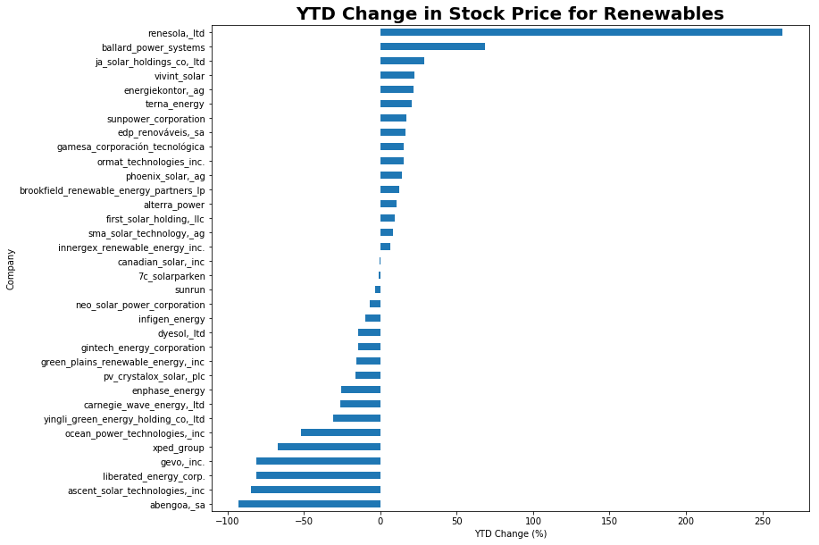
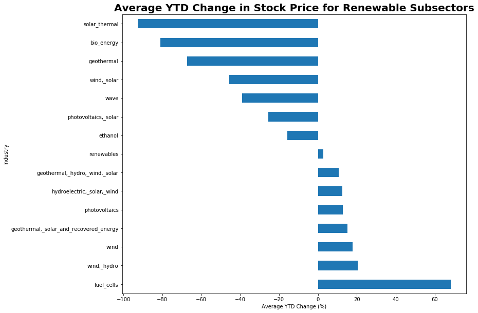
A somewhat unsurprising result, we see that stocks in fuel cells have been doing very well over the past year.
combined_data.groupby(['Industry'])['YTD'].mean().sort_values(ascending=False).plot(kind='barh', figsize = (12,10))
plt.title("Average YTD Change in Stock Price for Renewable Subsectors", fontsize=20, fontweight='bold')
plt.xlabel("Average YTD Change (%)")
plt.show()