Twitter - Financial News Scraper, VADER Sentiment Analysis
Twitter Live Feed
I’ve put together a simple script based on Sentdex’s great tutorials, highly recommend checking out here for some of the best Python tutorials out there.
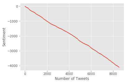
We can’t get a live feed going in a Jupyter Notebook, but if you run the below scripts, you can get a live updating version of twitter sentinment. The basic premise is to read in a stream of tweets, use the VADER sentiment analysis engine to assign a positive/negative score to each tweet, and then see how this cumulatively changes over time. It’s possible to use this to get a read on current sentiment behind certain topics. There even exists very high quality sentiment datasets available (with prices attached for access, unless you use Quantopian’s framework and can use in their notebooks).
from tweepy import Stream
from tweepy import OAuthHandler
from tweepy import StreamListener
import tweepy
import json
import ascii

ckey = "ckey"
csecret = "csecret"
atoken = "atoken"
asecret = "asecret"

analyzer = SentimentIntensityAnalyzer() # Use the VADER Sentiment Analyzer

class mslistener(StreamListener):

    def on_data(self, data):
        try:
            all_data = json.loads(data)
            tweet = all_data["text"]

            sentiment = analyzer.polarity_scores(tweet)['compound']
            if sentiment > 0:
                sentiment_value = "pos"
            else:
                sentiment_value = "neg"
            print(tweet, sentiment_value)

            output = open("twitter-currout.txt", "a")
            output.write(sentiment_value)
            output.write('\n')
            output.close()
        except:
            pass
        return(True)


    def on_error(self, status):
        print("Error:", status)

auth = OAuthHandler(ckey, csecret)
auth.set_access_token(atoken, asecret)

twitterStream = Stream(auth, listener = mslistener())
twitterStream.filter(track=["trump"])
RT @brianklaas: A neurosurgeon and a wedding planner walk into a bar...no just kidding they control US Federal Housing. https://t.co/MJHCwL… pos
Hmmm.  Is this it Rod? https://t.co/JNztNcmfZy neg
RT @RepBarbaraLee: What a bad decision. We worked so hard to re-open ties to Cuba – sickened to see this historic progress reversed. https:… neg
@NancyLynnNagy1 @ShaunKing And now trump n gop are trying to take away your healthcare yes? Such an informed choice… https://t.co/S97u9XtTB0 pos
@theblaze Remember obama told of Russia intervention in 2015 and Comey knew, and Clapper, no action. Obstruction of… https://t.co/nDb1qrkyy7 neg
RT @markberman: 12 hrs after Rosenstein bashes anonymous sources, Trump confirms he's under investigation, as reported in story based on...… neg
President Trump Decides To Not Deport “Dreamers” via Larry Ferlazzo's Websites of the Day… ... https://t.co/iMs6miyhfq neg
😂🤣 https://t.co/E6LTdPfx37 neg
...an this ! https://t.co/FM02Hlql28 neg
Trump contradicts his own account of Comey firing
Read here: https://t.co/uImoggyQCz https://t.co/FAf9m0lMfn neg
RT @Rockprincess818: This is the best one yet from Trump, so true.  describes with few words how perfectly insane it all is. #WitchHunt
htt… pos
RT @JackPosobiec: @realDonaldTrump Citizens will organize! Citizens for Trump! neg
RT @mediacrooks: The same pigs who supported every move to block Modi from entering the US? LOL! https://t.co/BvMNXwScg1 pos
Trump contradicts his own account of Comey firing
Read here: https://t.co/jWfZtYicJ4 https://t.co/2JJk9QlHRI neg
RT @hyped_resonance: Student Changes All Trump Shirts To Aphex Twin's Logo (Read More) https://t.co/TGIQEquKQa neg
RT @MSignorile: Fascinating that Trump claims it’s the media that “hates” his tweeting. They LOVE it. Gives them copy, stories. Undoes offi… pos
RT @mitchellvii: BAMM! Trump Administration Plans Summer Announcement of Wall Prototypes https://t.co/sFjSgBcbB3 neg
RT @benshapiro: I am amazed at Republicans tweeting out Trump supposedly ending DAPA while ignoring that he just basically made DACA perman… pos
RT @chelseaperetti: also a lot of us felt like when u openly asked russia to hack 2 help u win the election &then praised putin n lifte…  pos
RT @ForeignPolicy: Trump is pulling back Obama's outstretched hand to Cuba, alienating the State Department in the process. https://t.co/rd… pos
Could ignorance be Trump's  excuse? Who would deny it?-if Trump's ignorant, Trib's retarded!@ChicagoTribune https://t.co/fzqiHe40YJ neg
@evanstoner19 @Stuzy2813308004 Haha double standard bro. Comey screwed Clinton and that was "outrageous" but when h… https://t.co/oF5LWukVlh neg
RT @JrcheneyJohn: Trump fights back on Twitter👉Hillary destroyed phones, bleached emails ! Had real ties with Russia with URANIUM DEA…  neg
RT @thehill: Trump appoints family event planner to oversee New York federal housing: report https://t.co/CosGbfrJS7 https://t.co/jsEUO3KqX7 neg
RT @mitchellvii: In my experience following Trump, always seem most chaotic right before he closes. Has to be intentional tactic to confuse… neg
RT @WilDonnelly: Yes, don't listen to those anonymous sources that say Trump is under investigation. Wait until Trump confirms that…  pos
RT @RawStory: 'He's not in charge': US ally's defense minister says Mattis and Tillerson ignore Trump -- and make their own polic…  neg
RT @markmobility: Breaking: Trump Transition Team Orders Former Aides to Preserve Russia-Related Materials https://t.co/QGwflPsaz9 neg
Wait you have a boyfriend yet you support trump? U Poor thing PS is that a Ron Jeremy tat? https://t.co/wHPCXhFdoW neg
@BraddJaffy @MaxBoot Newt needs to be run out our town like all the Trump rats. pos
RT @Rockprincess818: So, Trump can't get Rosenstein to fire Mueller, and is plenty pissed about it. Fire Rosenstein ...go full scorched…  neg
RT @JYSexton: In the past few days my reporting has had me around more than a few Trump supporters, and what I've found has been surprising… pos
import matplotlib.pyplot as plt
import matplotlib.animation as animation
from matplotlib import style
import time
style.use("ggplot")

fig = plt.figure()
ax1 = fig.add_subplot(1,1,1)


def animate(i):
    pullData1 = open("twitter-currout.txt","r").read()

    lines1 = pullData1.split('\n')

    xar1 = []
    yar1 = []

    x1 = 0
    y1 = 0

    for l in lines1:
        x1 += 1
        if "pos" in l:
            y1 += 1
        elif "neg" in l:
            y1 -= 1

        xar1.append(x1)
        yar1.append(y1)

    ax1.clear()
    ax1.plot(xar1, yar1)
    ax1.set_ylabel("Sentiment")
    ax1.set_xlabel("Number of Tweets")

ani = animation.FuncAnimation(fig, animate, interval = 1000)

plt.show()
Analysis of Financial Twitter Data
https://github.com/Jefferson-Henrique/GetOldTweets-python retrieves historical tweets, and apply some cleaning in Excel to concatenate all the strings into a single string. We can retrieve historical tweets based on username for whoever we’re interested in i.e. Bloomberg, WSJ, Australian Financial Review, Washington Post, specific commentators etc. There’s really no limit to what we pull in except the time required to download all the data.
I use the line: python Exporter.py –username “username” –since 2010-01-01 –output “output.csv” in a Python 2.7 environment command line to generate each file.
I’ve only gone through a simple run-through here on Australian Financial Review (AFR), but there is so much data sitting on twitter waiting to be tested, so it’s an area which is going to keep growing. Primary difficulty is that tweets are often unstructured language, with poor formatting, lots of typos/errors which means considerable time and effort will need to go into cleaning the data.
import pandas as pd
import numpy as np
import matplotlib.pyplot as plt
def twitter_cleaner(file_path):
    df = pd.read_csv(file_path, delimiter=";")
    df = pd.DataFrame(df.ix[:,0].str.split(";").tolist())
    df = df.iloc[:, 0:10]
    df.columns = ["Username", "Date", "Retweets", "Favourites", "Tweet", "Geo", "Mentions", "Hastags", "ID", "Permalink"]
    df.Date = pd.to_datetime(df.Date)
    df['Short Date'] = df['Date'].apply(lambda x: x.date().strftime("%Y-%m-%d"))
    df.Tweet = df.Tweet.apply(lambda x: re.sub('http(.*)', "", x))

    return(df)

wsj_df = twitter_cleaner("C:/Users/Clint_PC/Downloads/GetOldTweets-python-master/output_wsj_clean.csv")
afr_df = twitter_cleaner("C:/Users/Clint_PC/Downloads/GetOldTweets-python-master/output_afr_clean.csv")
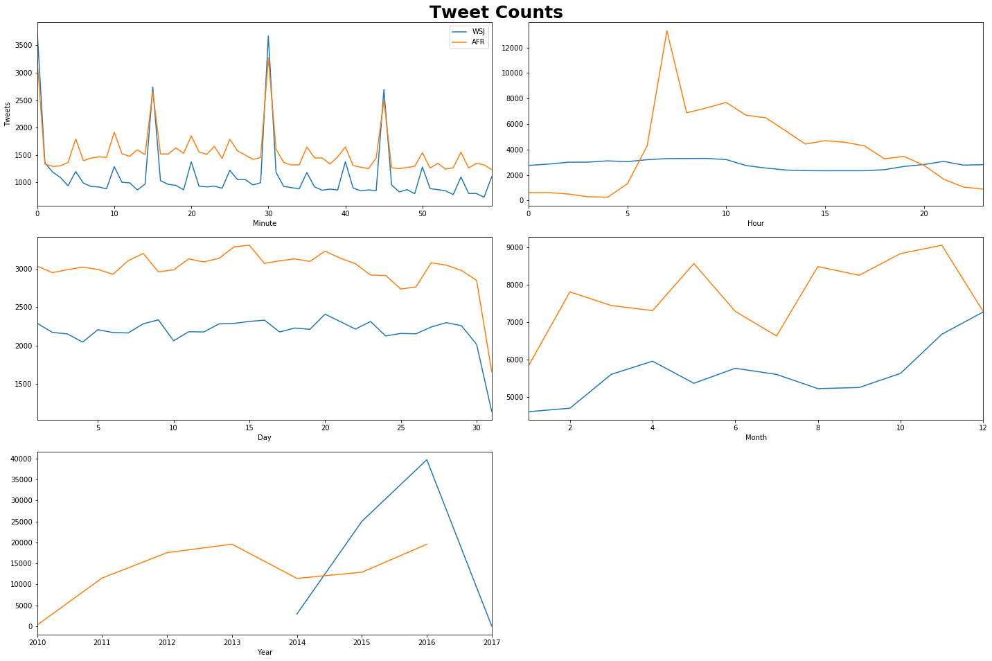
fig = plt.figure(figsize = (20,15))
plt.suptitle("Tweet Counts", size = 25, fontweight='bold')

plt.subplot(321)
ax=wsj_df.groupby(wsj_df.Date.map(lambda t: t.minute)).Tweet.count().plot()
afr_df.groupby(afr_df.Date.map(lambda t: t.minute)).Tweet.count().plot(ax=ax)
plt.xlabel("Minute")
plt.ylabel("Tweets")
ax.legend(["WSJ", "AFR"])

plt.subplot(322)
ax=wsj_df.groupby(wsj_df.Date.map(lambda t: t.hour)).Tweet.count().plot()
afr_df.groupby(afr_df.Date.map(lambda t: t.hour)).Tweet.count().plot(ax=ax)
plt.xlabel("Hour")

plt.subplot(323)
ax=wsj_df.groupby(wsj_df.Date.map(lambda t: t.day)).Tweet.count().plot()
afr_df.groupby(afr_df.Date.map(lambda t: t.day)).Tweet.count().plot(ax=ax)
plt.xlabel("Day")

plt.subplot(324)
ax=wsj_df.groupby(wsj_df.Date.map(lambda t: t.month)).Tweet.count().plot()
afr_df.groupby(afr_df.Date.map(lambda t: t.month)).Tweet.count().plot(ax=ax)
plt.xlabel("Month")

plt.subplot(325)
ax=wsj_df.groupby(wsj_df.Date.map(lambda t: t.year)).Tweet.count().plot()
afr_df.groupby(afr_df.Date.map(lambda t: t.year)).Tweet.count().plot(ax=ax)
plt.xlabel("Year")

plt.tight_layout(rect=[0, 0.1, 1, 0.97])
plt.show()
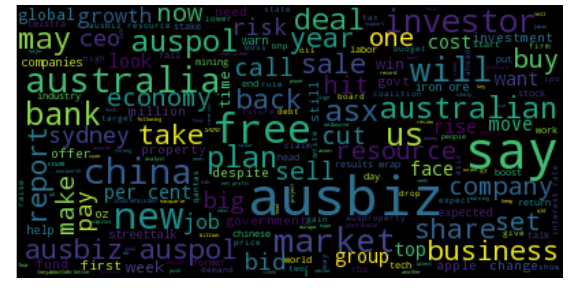
Combining Tweets into Daily Aggregates of Text
We run a bit of an iterative process here, where we use tf-idf to help us clean our dataset and get a view on some of the trending topics in each year. Our twitter data contains a whole bunch of irrelevant information such as twitter url’s, bit.ly url’s and what not.
from nltk.sentiment.vader import SentimentIntensityAnalyzer # VADER https://github.com/cjhutto/vaderSentiment
from nltk import tokenize

from sklearn.feature_extraction.text import CountVectorizer
from sklearn.linear_model import LogisticRegression
from nltk.corpus import stopwords
stop = set(stopwords.words('english'))
# Create a single string for each date (since we only want to look at word counts)
combined_tweets = afr_df.groupby(['Short Date']).Tweet.apply(lambda x: ' '.join(x).lower().strip()).reset_index()

combined_tweets.Tweet = combined_tweets.Tweet.str.replace("[", "")
combined_tweets.Tweet = combined_tweets.Tweet.str.replace("]", "")
combined_tweets.Tweet = combined_tweets.Tweet.str.replace("\\", "")
combined_tweets.Tweet = combined_tweets.Tweet.str.replace("@", "")
combined_tweets.Tweet = combined_tweets.Tweet.str.replace("\\,", "")
combined_tweets.Tweet = combined_tweets.Tweet.str.replace("\t", "")
combined_tweets.Tweet = combined_tweets.Tweet.str.replace("pic", "")
combined_tweets.Tweet = combined_tweets.Tweet.str.replace("'", "")
combined_tweets.Tweet = combined_tweets.Tweet.str.replace("sub", "")
combined_tweets.Tweet = combined_tweets.Tweet.str.replace("reqd", "")
combined_tweets.Tweet = combined_tweets.Tweet.str.replace("’", "")
combined_tweets.Tweet = combined_tweets.Tweet.str.replace("\"", "")
combined_tweets.Tweet = combined_tweets.Tweet.str.replace("…", "")

combined_tweets_string= str(tuple(combined_tweets.Tweet.tolist()))
#vectorizer = CountVectorizer()
#news_vect = vectorizer.build_tokenizer()(combined_tweets_string)
#word_counts = pd.DataFrame([[x,news_vect.count(x)] for x in set(news_vect)], columns = ['Word', 'Count'])
from wordcloud import WordCloud

# lower max_font_size
wordcloud = WordCloud(max_font_size=40).generate(combined_tweets_string)
plt.figure(figsize = (30,10))
plt.imshow(wordcloud, interpolation="bilinear")
plt.axis("off")
plt.show()
scores = pd.DataFrame(index = combined_tweets['Short Date'], columns = ['Compound', 'Positive', 'Negative', "Neutral"])
analyzer = SentimentIntensityAnalyzer() # Use the VADER Sentiment Analyzer
for j in range(1,combined_tweets.shape[0]):
tmp_neu = 0
tmp_neg = 0
tmp_pos = 0
tmp_comp = 0
text = afr_df.iloc[j,1]
if(str(text) == "nan"):
tmp_comp += 0
tmp_neg += 0
tmp_neu += 0
tmp_pos += 0
else:
vs = analyzer.polarity_scores(combined_tweets.iloc[j,1])
tmp_comp += vs['compound']
tmp_neg += vs['neg']
tmp_neu += vs['neu']
tmp_pos += vs['pos']
scores.iloc[j,] = [tmp_comp, tmp_pos, tmp_neg, tmp_neu]
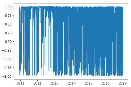
scores = scores.apply(pd.to_numeric)
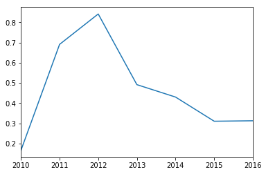
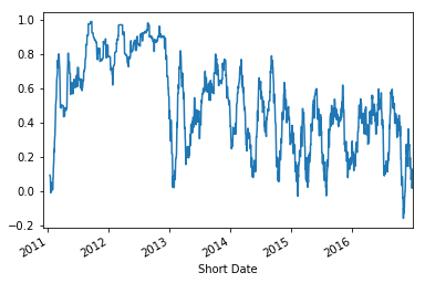
We can see some interesting patterns in looking at the compound sentiment of the AFR twitter account. In particular we see that the account is on average positive, but has been on a slow downward trend post 2012.
scores.index = pd.to_datetime(scores.index)
scores['year'] = scores.index.map(lambda t: t.year)
scores['month'] = scores.index.map(lambda t: t.month)
plt.plot(scores.Compound)
plt.tight_layout()
plt.show()
scores.groupby([scores.index.map(lambda t: t.year)])['Compound'].mean().plot()
plt.show()
scores['Compound'].rolling(30).mean().plot()
plt.show()
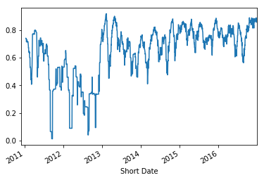
scores['Compound'].rolling(30).std().plot()
plt.show()
We can apply some tf-idf to analyse key topics in our twitter sets, as well as allowing us the ability to filter out certain unclean data (i.e. grammar, urls). We see that tf-idf does a decent job at pulling out some of the key topics from each year.
- 2011: Eurozone/Greek Debt Crisis
- 2012: US Fiscal Cliff
- 2014: Sydney Siege
- 2015: Paris Attacks
We also can see the type of noise which flows through a twitter language analysis, things like “frsunday” = Financial Review Sunday, dates, headlines, and twitter hashtags. These are things which need to be dealt with for more advanced data analysis.
import math
from textblob import TextBlob as tb

def tf(word, blob):
    return blob.words.count(word) / len(blob.words)

def n_containing(word, bloblist):
    return sum(1 for blob in bloblist if word in blob.words)

def idf(word, bloblist):
    return math.log(len(bloblist) / (1 + n_containing(word, bloblist)))

def tfidf(word, blob, bloblist):
    return tf(word, blob) * idf(word, bloblist)

docs = combined_tweets
docs.set_index('Short Date', inplace=True)


doc_2010 = docs[(docs.index >= "2010-11-01") & (docs.index < "2011-01-01")].Tweet.str.cat(sep = ' ').lower()
doc_2011 = docs[(docs.index >= "2011-11-01") & (docs.index < "2012-01-01")].Tweet.str.cat(sep = ' ').lower()
doc_2012 = docs[(docs.index >= "2012-11-01") & (docs.index < "2013-01-01")].Tweet.str.cat(sep = ' ').lower()
doc_2013 = docs[(docs.index >= "2013-11-01") & (docs.index < "2014-01-01")].Tweet.str.cat(sep = ' ').lower()
doc_2014 = docs[(docs.index >= "2014-11-01") & (docs.index < "2015-01-01")].Tweet.str.cat(sep = ' ').lower()
doc_2015 = docs[(docs.index >= "2015-11-01") & (docs.index < "2016-01-01")].Tweet.str.cat(sep = ' ').lower()
doc_2016 =docs[(docs.index >= "2016-06-01") & (docs.index < "2017-01-01")].Tweet.str.cat(sep = ' ').lower()

#bloblist = [tb(doc_2008), tb(doc_2009), tb(doc_2010), tb(doc_2011), tb(doc_2012), tb(doc_2013), tb(doc_2014)
#           , tb(doc_2015), tb(doc_2016)]

bloblist = [tb(doc_2010), tb(doc_2011), tb(doc_2012), tb(doc_2013), tb(doc_2014), tb(doc_2015), tb(doc_2016)]

for i, blob in enumerate(bloblist):
    print("Top words in document year {}".format(i + 2010))
    scores = {word: tfidf(word, blob, bloblist) for word in (set(blob.words)-stop)}
    sorted_words = sorted(scores.items(), key=lambda x: x[1], reverse=True)
    for word, score in sorted_words[:5]:
        print("\tWord: {}, TF-IDF: {}".format(word, round(score, 5)))
Top words in document year 2010
	Word: marketwrap5pm, TF-IDF: 0.00202
	Word: dealbook, TF-IDF: 0.00154
	Word: riversdale, TF-IDF: 0.00137
	Word: gainers, TF-IDF: 0.00103
	Word: req, TF-IDF: 0.00101
Top words in document year 2011
	Word: csg, TF-IDF: 0.00057
	Word: eurozone, TF-IDF: 0.00055
	Word: onesteel, TF-IDF: 0.00049
	Word: greece, TF-IDF: 0.0004
	Word: ir, TF-IDF: 0.00039
Top words in document year 2012
	Word: juliagillard, TF-IDF: 0.00042
	Word: cliff, TF-IDF: 0.00039
	Word: ausproperty, TF-IDF: 0.00037
	Word: ausecon, TF-IDF: 0.00036
	Word: fiscalcliff, TF-IDF: 0.00034
Top words in document year 2013
	Word: wcb, TF-IDF: 0.00097
	Word: warrnambool, TF-IDF: 0.00092
	Word: taper, TF-IDF: 0.00058
	Word: ausecon, TF-IDF: 0.00057
	Word: frsunday, TF-IDF: 0.00055
Top words in document year 2014
	Word: sydneysiege, TF-IDF: 0.00101
	Word: g20brisbane, TF-IDF: 0.00064
	Word: frsunday, TF-IDF: 0.00061
	Word: medibank, TF-IDF: 0.00057
	Word: round-up, TF-IDF: 0.00047
Top words in document year 2015
	Word: turnbull, TF-IDF: 0.00084
	Word: parisattacks, TF-IDF: 0.00072
	Word: 2016, TF-IDF: 0.00065
	Word: streettalk, TF-IDF: 0.00063
	Word: philabaker, TF-IDF: 0.00059
To Explore
- Sentiment with multiple twitter accounts
- Correlation with markets