League of Legends Exploration

An incredibly popular RTS game, League of Legends is an interesting combination of player mechanics, individual skill and teamwork. Here we investigate a dataset of LoL matches and see whether we can use any of it to predict a winner!

Pre-Processing

import pandas as pd 
import numpy as np
import matplotlib.pyplot as plt
import json as json

import seaborn as sns

df = pd.read_csv(r"D:\Downloads\Coding\league-of-legends\games.csv")
champions = pd.read_json(r"D:\Downloads\Coding\league-of-legends\champion_info.json")
spells = pd.read_json(r"D:\Downloads\Coding\league-of-legends\summoner_spell_info.json")

df.head()

	gameId	gameDuration	seasonId	firstBlood	firstTower	firstInhibitor	firstBaron	firstDragon	firstRiftHerald	...	t2_towerKills	t2_dragonKills	t2_riftHeraldKills	t2_ban1	t2_ban2	t2_ban3	t2_ban4	t2_ban5
0	3326086514	1949	9	0	1	1	1	1	0	...	5	1	1	114	67	43	16	51
1	3229566029	1851	9	1	1	1	0	1	1	...	2	0	0	11	67	238	51	420
2	3327363504	1493	9	0	1	1	1	0	0	...	2	1	0	157	238	121	57	28
3	3326856598	1758	9	1	1	1	1	1	0	...	0	0	0	164	18	141	40	51
4	3330080762	2094	9	0	1	1	1	1	0	...	3	1	0	86	11	201	122	18

5 rows × 60 columns

df.info()

<class 'pandas.core.frame.DataFrame'>
RangeIndex: 51536 entries, 0 to 51535
Data columns (total 60 columns):
gameId                51536 non-null int64
gameDuration          51536 non-null int64
seasonId              51536 non-null int64
winner                51536 non-null int64
firstBlood            51536 non-null int64
firstTower            51536 non-null int64
firstInhibitor        51536 non-null int64
firstBaron            51536 non-null int64
firstDragon           51536 non-null int64
firstRiftHerald       51536 non-null int64
t1_champ1id           51536 non-null int64
t1_champ1_sum1        51536 non-null int64
t1_champ1_sum2        51536 non-null int64
t1_champ2id           51536 non-null int64
t1_champ2_sum1        51536 non-null int64
t1_champ2_sum2        51536 non-null int64
t1_champ3id           51536 non-null int64
t1_champ3_sum1        51536 non-null int64
t1_champ3_sum2        51536 non-null int64
t1_champ4id           51536 non-null int64
t1_champ4_sum1        51536 non-null int64
t1_champ4_sum2        51536 non-null int64
t1_champ5id           51536 non-null int64
t1_champ5_sum1        51536 non-null int64
t1_champ5_sum2        51536 non-null int64
t1_towerKills         51536 non-null int64
t1_inhibitorKills     51536 non-null int64
t1_baronKills         51536 non-null int64
t1_dragonKills        51536 non-null int64
t1_riftHeraldKills    51536 non-null int64
t1_ban1               51536 non-null int64
t1_ban2               51536 non-null int64
t1_ban3               51536 non-null int64
t1_ban4               51536 non-null int64
t1_ban5               51536 non-null int64
t2_champ1id           51536 non-null int64
t2_champ1_sum1        51536 non-null int64
t2_champ1_sum2        51536 non-null int64
t2_champ2id           51536 non-null int64
t2_champ2_sum1        51536 non-null int64
t2_champ2_sum2        51536 non-null int64
t2_champ3id           51536 non-null int64
t2_champ3_sum1        51536 non-null int64
t2_champ3_sum2        51536 non-null int64
t2_champ4id           51536 non-null int64
t2_champ4_sum1        51536 non-null int64
t2_champ4_sum2        51536 non-null int64
t2_champ5id           51536 non-null int64
t2_champ5_sum1        51536 non-null int64
t2_champ5_sum2        51536 non-null int64
t2_towerKills         51536 non-null int64
t2_inhibitorKills     51536 non-null int64
t2_baronKills         51536 non-null int64
t2_dragonKills        51536 non-null int64
t2_riftHeraldKills    51536 non-null int64
t2_ban1               51536 non-null int64
t2_ban2               51536 non-null int64
t2_ban3               51536 non-null int64
t2_ban4               51536 non-null int64
t2_ban5               51536 non-null int64
dtypes: int64(60)
memory usage: 23.6 MB

df.describe()

	gameId	gameDuration	seasonId	winner	firstBlood	firstTower	firstInhibitor	firstBaron	firstDragon	firstRiftHerald	...	t2_towerKills	t2_inhibitorKills	t2_baronKills	t2_dragonKills	t2_riftHeraldKills	t2_ban1	t2_ban2	t2_ban3	t2_ban4	t2_ban5
count	5.153600e+04	51536.000000	51536.0	51536.000000	51536.000000	51536.000000	51536.000000	51536.000000	51536.000000	51536.000000	...	51536.000000	51536.000000	51536.000000	51536.000000	51536.000000	51536.000000	51536.000000	51536.000000	51536.000000	51536.000000
mean	3.306218e+09	1832.433658	9.0	0.493577	0.507141	0.502134	0.447765	0.286654	0.479471	0.251416	...	5.549849	0.985078	0.414565	1.404397	0.240220	108.203605	107.957991	108.686666	108.636196	108.081031
std	2.946137e+07	511.935772	0.0	0.499964	0.499954	0.500000	0.497269	0.452203	0.499583	0.433832	...	3.860701	1.256318	0.613800	1.224289	0.427221	102.538299	102.938916	102.592143	103.356702	102.762418
min	3.214824e+09	190.000000	9.0	0.000000	0.000000	0.000000	0.000000	0.000000	0.000000	0.000000	...	0.000000	0.000000	0.000000	0.000000	0.000000	-1.000000	-1.000000	-1.000000	-1.000000	-1.000000
25%	3.292212e+09	1531.000000	9.0	0.000000	0.000000	0.000000	0.000000	0.000000	0.000000	0.000000	...	2.000000	0.000000	0.000000	0.000000	0.000000	38.000000	37.000000	38.000000	38.000000	38.000000
50%	3.319969e+09	1833.000000	9.0	0.000000	1.000000	1.000000	0.000000	0.000000	0.000000	0.000000	...	6.000000	0.000000	0.000000	1.000000	0.000000	90.000000	90.000000	90.000000	90.000000	90.000000
75%	3.327097e+09	2148.000000	9.0	1.000000	1.000000	1.000000	1.000000	1.000000	1.000000	1.000000	...	9.000000	2.000000	1.000000	2.000000	0.000000	141.000000	141.000000	141.000000	141.000000	141.000000
max	3.331833e+09	4728.000000	9.0	1.000000	1.000000	1.000000	1.000000	1.000000	1.000000	1.000000	...	11.000000	10.000000	4.000000	6.000000	1.000000	516.000000	516.000000	516.000000	516.000000	516.000000

8 rows × 60 columns

EDA

We can perform some basic manipulations to get an insight into the frequency with which differenct champions & summoner spells are selected, as well as the differences in selection between the two teams.

Most common champion picks
Most common team picks
Most common pairs
Most common spells
Most common champion + spells

# Convert from an ID to a name
champ_names11 = [champions.ix[y][0]['name'] for y in df.t1_champ1id]
champ_names12 = [champions.ix[y][0]['name'] for y in df.t1_champ2id]
champ_names13 = [champions.ix[y][0]['name'] for y in df.t1_champ3id]
champ_names14 = [champions.ix[y][0]['name'] for y in df.t1_champ4id]
champ_names15 = [champions.ix[y][0]['name'] for y in df.t1_champ5id]

champ_names21 = [champions.ix[y][0]['name'] for y in df.t2_champ1id]
champ_names22 = [champions.ix[y][0]['name'] for y in df.t2_champ2id]
champ_names23 = [champions.ix[y][0]['name'] for y in df.t2_champ3id]
champ_names24 = [champions.ix[y][0]['name'] for y in df.t2_champ4id]
champ_names25 = [champions.ix[y][0]['name'] for y in df.t2_champ5id]

c11 = pd.DataFrame(np.column_stack([champ_names11, np.repeat(1, len(df)), np.repeat(1, len(df))]), 
            columns=["name", "team", "champ"])
c12 = pd.DataFrame(np.column_stack([champ_names12, np.repeat(1, len(df)), np.repeat(2, len(df))]), 
            columns=["name", "team", "champ"])
c13 = pd.DataFrame(np.column_stack([champ_names13, np.repeat(1, len(df)), np.repeat(3, len(df))]), 
            columns=["name", "team", "champ"])
c14 = pd.DataFrame(np.column_stack([champ_names14, np.repeat(1, len(df)), np.repeat(4, len(df))]), 
            columns=["name", "team", "champ"])
c15 = pd.DataFrame(np.column_stack([champ_names15, np.repeat(1, len(df)), np.repeat(5, len(df))]), 
            columns=["name", "team", "champ"])

c21 = pd.DataFrame(np.column_stack([champ_names21, np.repeat(2, len(df)), np.repeat(1, len(df))]), 
            columns=["name", "team", "champ"])
c22 = pd.DataFrame(np.column_stack([champ_names22, np.repeat(2, len(df)), np.repeat(2, len(df))]), 
            columns=["name", "team", "champ"])
c23 = pd.DataFrame(np.column_stack([champ_names23, np.repeat(2, len(df)), np.repeat(3, len(df))]), 
            columns=["name", "team", "champ"])
c24 = pd.DataFrame(np.column_stack([champ_names24, np.repeat(2, len(df)), np.repeat(4, len(df))]), 
            columns=["name", "team", "champ"])
c25 = pd.DataFrame(np.column_stack([champ_names25, np.repeat(2, len(df)), np.repeat(5, len(df))]), 
            columns=["name", "team", "champ"])

comb_names = pd.DataFrame(np.vstack([c11, c12, c13, c14, c15, c21, c22, c23, c24, c25]),
                         columns=["name", "team", "champ"])

# Convert from an ID to a name
spells_names111 = [spells.ix[y][0]['name'] for y in df.t1_champ1_sum1]
spells_names112 = [spells.ix[y][0]['name'] for y in df.t1_champ1_sum2]
spells_names121 = [spells.ix[y][0]['name'] for y in df.t1_champ2_sum1]
spells_names122 = [spells.ix[y][0]['name'] for y in df.t1_champ2_sum2]
spells_names131 = [spells.ix[y][0]['name'] for y in df.t1_champ3_sum1]
spells_names132 = [spells.ix[y][0]['name'] for y in df.t1_champ3_sum2]
spells_names141 = [spells.ix[y][0]['name'] for y in df.t1_champ4_sum1]
spells_names142 = [spells.ix[y][0]['name'] for y in df.t1_champ4_sum2]
spells_names151 = [spells.ix[y][0]['name'] for y in df.t1_champ5_sum1]
spells_names152 = [spells.ix[y][0]['name'] for y in df.t1_champ5_sum2]

spells_names211 = [spells.ix[y][0]['name'] for y in df.t2_champ1_sum1]
spells_names212 = [spells.ix[y][0]['name'] for y in df.t2_champ1_sum2]
spells_names221 = [spells.ix[y][0]['name'] for y in df.t2_champ2_sum1]
spells_names222 = [spells.ix[y][0]['name'] for y in df.t2_champ2_sum2]
spells_names231 = [spells.ix[y][0]['name'] for y in df.t2_champ3_sum1]
spells_names232 = [spells.ix[y][0]['name'] for y in df.t2_champ3_sum2]
spells_names241 = [spells.ix[y][0]['name'] for y in df.t2_champ4_sum1]
spells_names242 = [spells.ix[y][0]['name'] for y in df.t2_champ4_sum2]
spells_names251 = [spells.ix[y][0]['name'] for y in df.t2_champ5_sum1]
spells_names252 = [spells.ix[y][0]['name'] for y in df.t2_champ5_sum2]

t1s1 = pd.DataFrame(np.column_stack([spells_names111, spells_names112, np.repeat(1, len(df)), np.repeat(1, len(df))]), 
            columns=["sum1", "sum2", "team", "champ"])
t1s2 = pd.DataFrame(np.column_stack([spells_names121, spells_names122, np.repeat(1, len(df)), np.repeat(2, len(df))]), 
            columns=["sum1", "sum2", "team", "champ"])
t1s3 = pd.DataFrame(np.column_stack([spells_names131, spells_names132, np.repeat(1, len(df)), np.repeat(3, len(df))]), 
            columns=["sum1", "sum2", "team", "champ"])
t1s4 = pd.DataFrame(np.column_stack([spells_names141, spells_names142, np.repeat(1, len(df)), np.repeat(4, len(df))]), 
            columns=["sum1", "sum2", "team", "champ"])
t1s5 = pd.DataFrame(np.column_stack([spells_names151, spells_names152, np.repeat(1, len(df)), np.repeat(5, len(df))]), 
            columns=["sum1", "sum2", "team", "champ"])

t2s1 = pd.DataFrame(np.column_stack([spells_names211, spells_names212, np.repeat(2, len(df)), np.repeat(1, len(df))]), 
            columns=["sum1", "sum2", "team", "champ"])
t2s2 = pd.DataFrame(np.column_stack([spells_names221, spells_names222, np.repeat(2, len(df)), np.repeat(2, len(df))]), 
            columns=["sum1", "sum2", "team", "champ"])
t2s3 = pd.DataFrame(np.column_stack([spells_names231, spells_names232, np.repeat(2, len(df)), np.repeat(3, len(df))]), 
            columns=["sum1", "sum2", "team", "champ"])
t2s4 = pd.DataFrame(np.column_stack([spells_names241, spells_names242, np.repeat(2, len(df)), np.repeat(4, len(df))]), 
            columns=["sum1", "sum2", "team", "champ"])
t2s5 = pd.DataFrame(np.column_stack([spells_names251, spells_names252, np.repeat(2, len(df)), np.repeat(5, len(df))]), 
            columns=["sum1", "sum2", "team", "champ"])

comb_spells = pd.DataFrame(np.vstack([t1s1, t1s2, t1s3, t1s4, t1s5,
                                     t2s1, t2s2, t2s3, t2s4, t2s5]), 
                          columns=["sum1", "sum2", "team", "champ"])

# Aggregate all info into a single dataframe
all_names = pd.merge(comb_names, comb_spells, left_index=True, right_index=True)
all_names = all_names.drop(["team_y", "champ_y"], axis=1)

Champion Selections

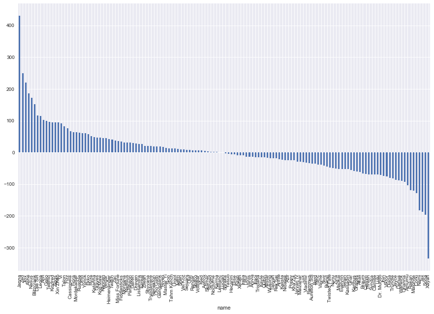
Here we map out both the difference in selections between the two teams, as well as the total frequency of champion selection.

Interestingly we see that Janna and Xayah have the most dispairty between the two teams. Perhaps they are both good counters to each other and so if one team sees the other being chosen, the opposing team counters. In the middle of the pack with little to no difference we see picks such as Lucian, LeBlanc, Karma, Soraka and Yasuo.

plt.figure(figsize=(15,10))
test = all_names.groupby(["name", "team_x"])["champ_x"].count()
test = test.unstack()
test["diff"] = test.ix[:, 0] - test.ix[:, 1]
test["diff"].sort_values(ascending=False).plot(kind="bar")
plt.show()

png

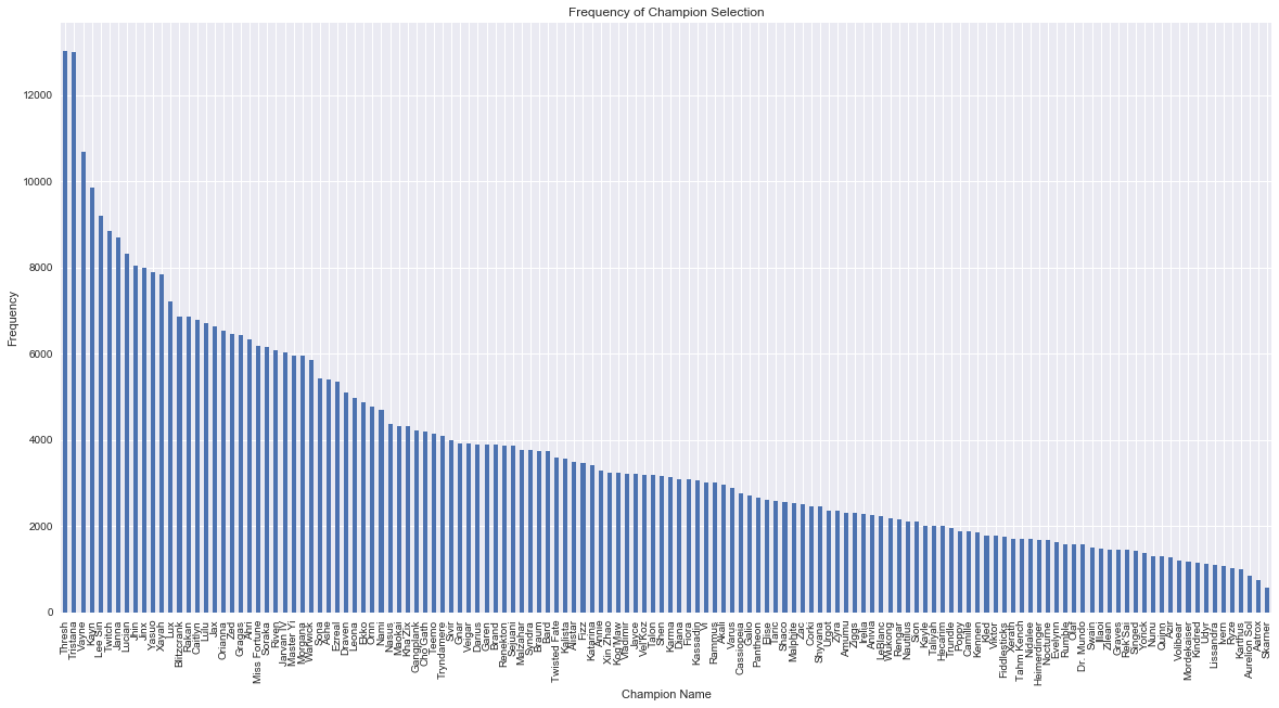
In terms of total frequency, we see Thresh and Tristana fighting it out for first place, with them being followed up by Vayne, Kayn and Lee Sin. No surprises here given the popularity of these champions.

plt.figure(figsize=(20,10))
all_names.groupby(["name"])["name"].count().sort_values(ascending=False).plot(kind="bar")
plt.ylabel("Frequency")
plt.xlabel("Champion Name")
plt.title("Frequency of Champion Selection")
plt.show()

png

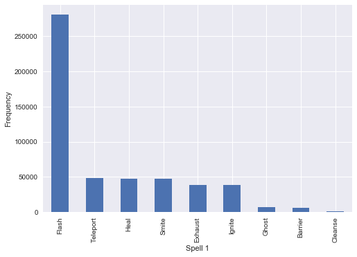
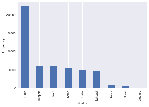
Summoner Spells

We conduct a similar process as above, and exmaine the most frequently used summoner spells and pairings with champions. Not unsurprisingly Flash tops the list in both cases. It looks like Ghost, Barrier and Cleanse are seen as the worst performing spells and rarely picked.

all_names.groupby(["sum1"])["sum1"].count().sort_values(ascending=False).plot(kind="bar")
plt.xlabel("Spell 1")
plt.ylabel("Frequency")
plt.show()

all_names.groupby(["sum2"])["sum2"].count().sort_values(ascending=False).plot(kind="bar")
plt.xlabel("Spell 2")
plt.ylabel("Frequency")
plt.show()

png

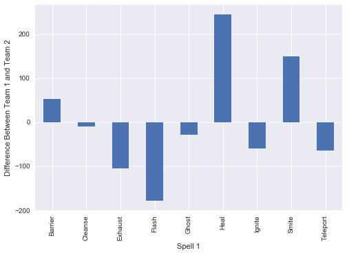
sum1_diff = all_names.groupby(["sum1", "team_x"])["sum1"].count().unstack()
sum1_diff["diff"] = sum1_diff.ix[:,0] - sum1_diff.ix[:,1]
sum1_diff["diff"].plot(kind="bar")
plt.ylabel("Difference Between Team 1 and Team 2")
plt.xlabel("Spell 1")
plt.show()

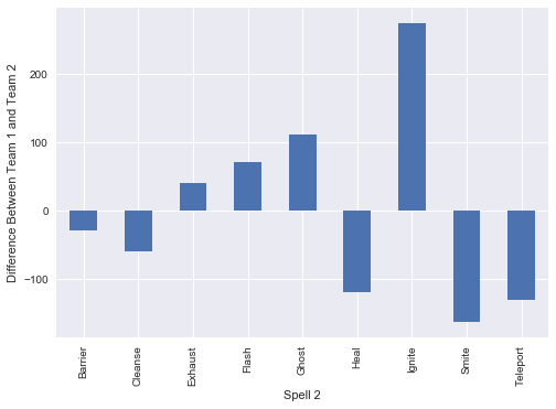
sum2_diff = all_names.groupby(["sum2", "team_x"])["sum2"].count().unstack()
sum2_diff["diff"] = sum2_diff.ix[:,0] - sum2_diff.ix[:,1]
sum2_diff["diff"].plot(kind="bar")
plt.ylabel("Difference Between Team 1 and Team 2")
plt.xlabel("Spell 2")
plt.show()

png

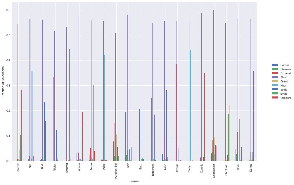
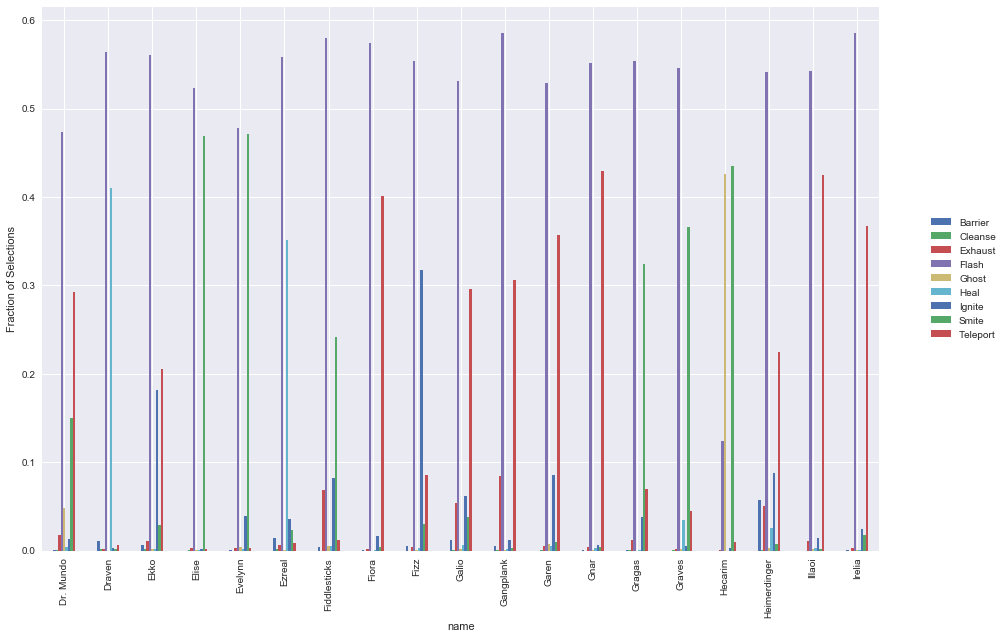
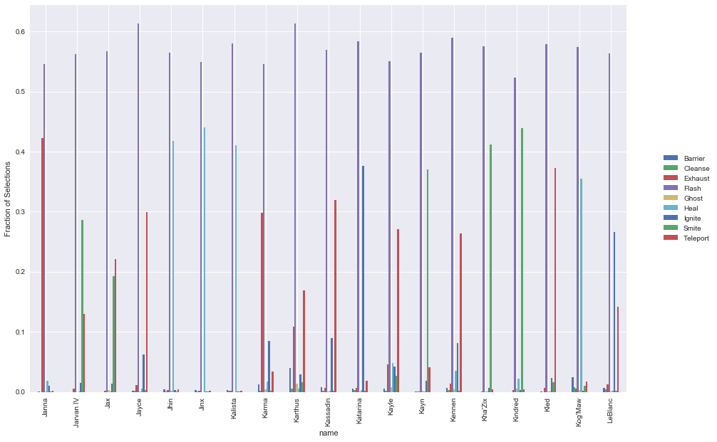
An interesting question is what are the most common spell selections for each champion. We expect that there would be considerable variation in spell selections, depending on both individual playstyle as well as the category that the champion falls into. To do this, we can simply aggregate up all the champions & spells, and then normalise across each champion to get the ratios that each one selects.

Some points of interest:

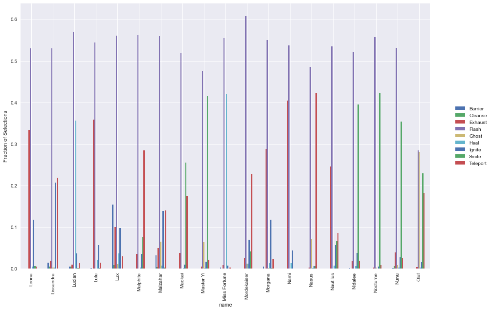
Average ratio of flash is ~55-60%
Hecarim has a substantially lower ratio of flash, given his special which allows him to escape quickly
Olaf also has a substantially lower ratio of flash
Also appears to be a fairly consistent ratio of the second preferred spell across most champions

champ_spell_comb = all_names.groupby(["name", "sum1"])["name"].count().unstack().fillna(0)
champ_spell_comb = champ_spell_comb.div(champ_spell_comb.sum(axis=1), axis=0) # normalising

champ_spell_comb.ix[0:20, :].plot(kind="bar", figsize=(15,10))
plt.ylabel("Fraction of Selections")
plt.legend(loc='center right', bbox_to_anchor=(1.15, 0.5))
plt.show()

champ_spell_comb.ix[21:40, :].plot(kind="bar", figsize=(15,10))
plt.ylabel("Fraction of Selections")
plt.legend(loc='center right', bbox_to_anchor=(1.15, 0.5))
plt.show()

champ_spell_comb.ix[41:60, :].plot(kind="bar", figsize=(15,10))
plt.ylabel("Fraction of Selections")
plt.legend(loc='center right', bbox_to_anchor=(1.15, 0.5))
plt.show()

champ_spell_comb.ix[61:80, :].plot(kind="bar", figsize=(15,10))
plt.ylabel("Fraction of Selections")
plt.legend(loc='center right', bbox_to_anchor=(1.15, 0.5))
plt.show()

champ_spell_comb.ix[81:100, :].plot(kind="bar", figsize=(15,10))
plt.ylabel("Fraction of Selections")
plt.legend(loc='center right', bbox_to_anchor=(1.15, 0.5))
plt.show()

champ_spell_comb.ix[101:128, :].plot(kind="bar", figsize=(15,10))
plt.ylabel("Fraction of Selections")
plt.legend(loc='center right', bbox_to_anchor=(1.15, 0.5))
plt.show()

png

Predictive Analysis

Now that we’ve pulled apart the data, what’s more interesting is seeing whether we can use it to predict the winner of a game.

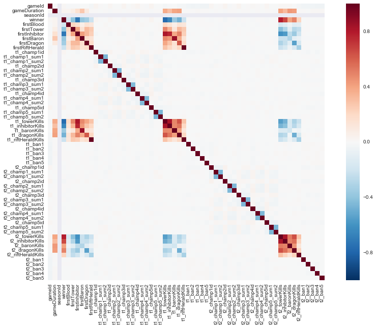
From the heatmap below, we see that there are very obvious clusters of correlated variables:

First game objectives
Total number of objective kills

These are not unsurprising as a team who is doing good/bad will likely of opposing levels of objectives/kills.

corrmat = df.corr()
plt.figure(figsize = (15,10))
sns.heatmap(corrmat, square=True)
plt.show()

png

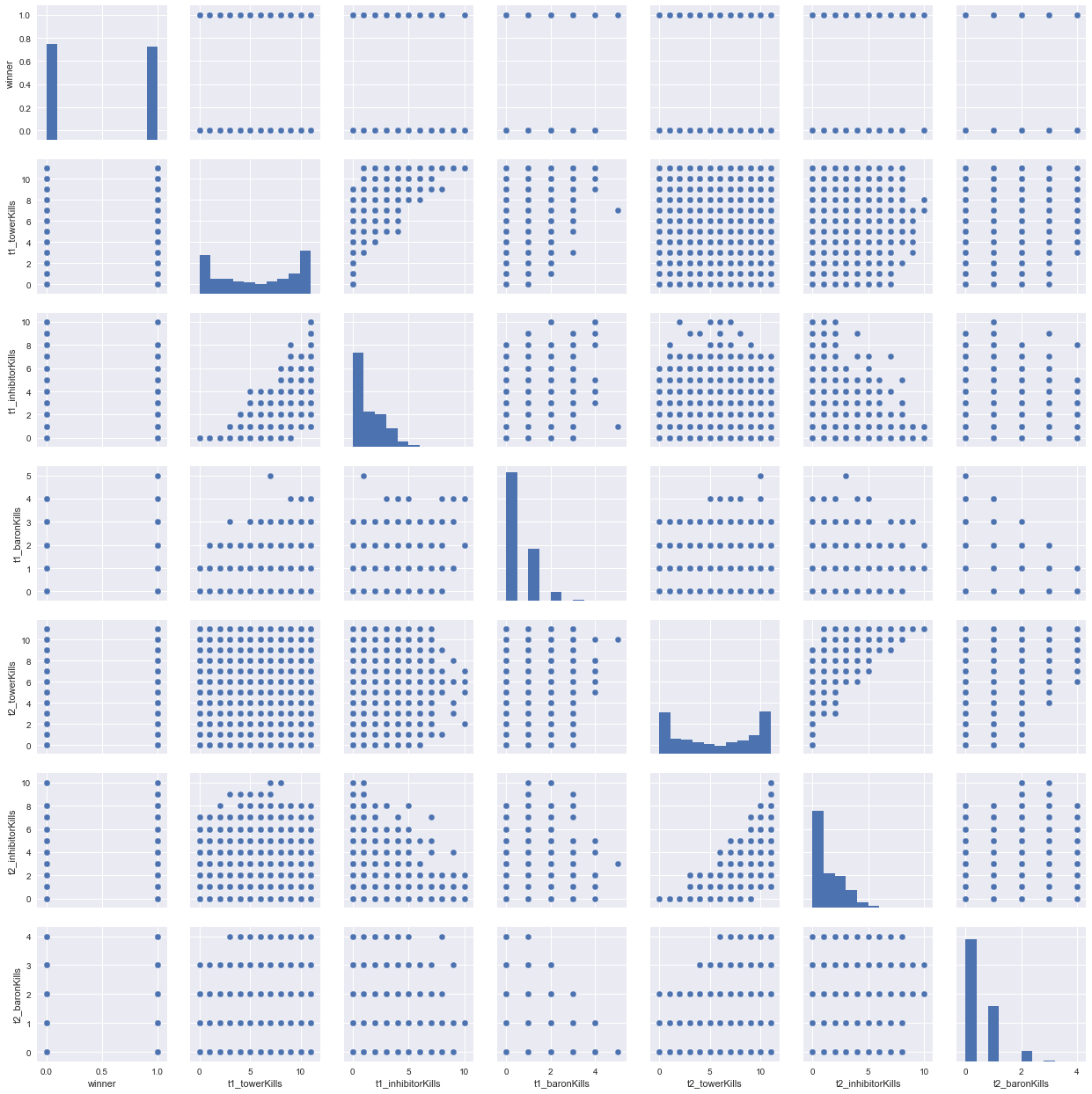
cols = ['winner','t1_towerKills', 't1_inhibitorKills', 't1_baronKills', 't2_towerKills', 't2_inhibitorKills', 't2_baronKills',]

sns.pairplot(df[cols])
plt.show()

png

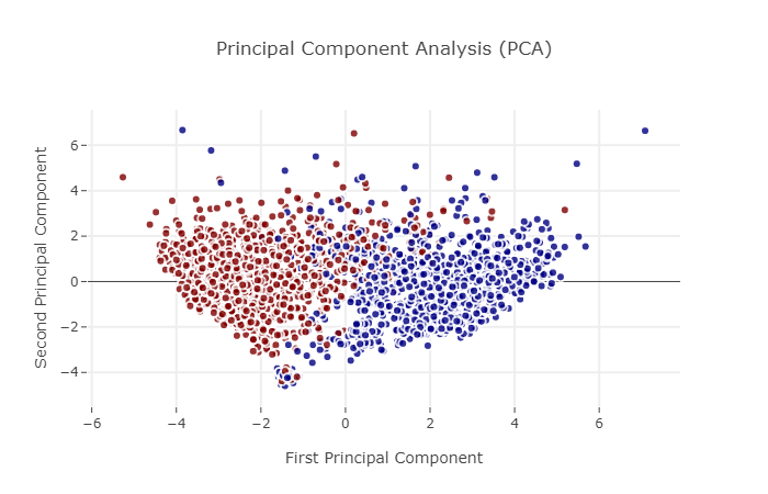
Structural Analysis

We can do some basic PCA and K-Means clustering to see if there is any obvious structure which exists in our dataset. We should also be clear that we are working with the dataset that does include endgame statistics… i.e. we should expect fairly high predictive strength. We will investigate later a prediction using variables only known at the start of a match.

import plotly.offline as py
py.init_notebook_mode(connected=True)
import plotly.graph_objs as go
import plotly.tools as tls

from sklearn.decomposition import PCA
from sklearn.preprocessing import StandardScaler

X = df.drop(['gameId', 'seasonId', 'winner'], 1)
y = df['winner']

X_std = StandardScaler().fit_transform(X)
n_components = 5
X_std = X_std[:2000]
pca = PCA(n_components=n_components).fit(X_std)
Target = y[:2000]
X_5d = pca.transform(X_std)

trace0 = go.Scatter(
    x = X_5d[:,0],
    y = X_5d[:,1],
    name = Target,
    hoveron = Target,
    mode = 'markers',
    text = Target,
    showlegend = False,
    marker = dict(
        size = 8,
        color = Target,
        colorscale ='Jet',
        showscale = False,
        line = dict(
            width = 2,
            color = 'rgb(255, 255, 255)'
        ),
        opacity = 0.8
    )
)
data = [trace0]

layout = go.Layout(
    title= 'Principal Component Analysis (PCA)',
    hovermode= 'closest',
    xaxis= dict(
         title= 'First Principal Component',
        ticklen= 5,
        zeroline= False,
        gridwidth= 2,
    ),
    yaxis=dict(
        title= 'Second Principal Component',
        ticklen= 5,
        gridwidth= 2,
    ),
    showlegend= True
)


fig = dict(data=data, layout=layout)
py.iplot(fig, filename='styled-scatter')

png

from sklearn.cluster import KMeans # KMeans clustering 
kmeans = KMeans(n_clusters=2)
X_clustered = kmeans.fit_predict(X_5d)

trace_Kmeans = go.Scatter(x=X_5d[:, 0], y= X_5d[:, 1], mode="markers",
                    showlegend=False,
                    marker=dict(
                            size=8,
                            color = X_clustered,
                            colorscale = 'Portland',
                            showscale=False, 
                            line = dict(
            width = 2,
            color = 'rgb(255, 255, 255)'
        )
                   ))

layout = go.Layout(
    title= 'KMeans Clustering',
    hovermode= 'closest',
    xaxis= dict(
         title= 'First Principal Component',
        ticklen= 5,
        zeroline= False,
        gridwidth= 2,
    ),
    yaxis=dict(
        title= 'Second Principal Component',
        ticklen= 5,
        gridwidth= 2,
    ),
    showlegend= True
)

data = [trace_Kmeans]
fig1 = dict(data=data, layout= layout)
# fig1.append_trace(contour_list)
py.iplot(fig1, filename="svm")

png

from sklearn.manifold import TSNE

tsne = TSNE()
tsne_results = tsne.fit_transform(X_std) 

traceTSNE = go.Scatter(
    x = tsne_results[:,0],
    y = tsne_results[:,1],
    name = Target,
     hoveron = Target,
    mode = 'markers',
    text = Target,
    showlegend = True,
    marker = dict(
        size = 8,
        color = Target,
        colorscale ='Jet',
        showscale = False,
        line = dict(
            width = 2,
            color = 'rgb(255, 255, 255)'
        ),
        opacity = 0.8
    )
)
data = [traceTSNE]

layout = dict(title = 'TSNE (T-Distributed Stochastic Neighbour Embedding)',
              hovermode= 'closest',
              yaxis = dict(zeroline = False),
              xaxis = dict(zeroline = False),
              showlegend= False,

             )

fig = dict(data=data, layout=layout)
py.iplot(fig, filename='styled-scatter')

png

The above three techniques demonstrate that there is a pretty clear structural differentiation between winning and losing. This bodes well for running some machine learning techniques across the dataset.

As seen below, the scores we get are all in excess of 90%. This is not unexpected given the level of data which is available and the fact that it is end game data.

#Preprocessing
from sklearn.model_selection import train_test_split
from sklearn.preprocessing import StandardScaler

#Algos
from sklearn.linear_model import LogisticRegression
from sklearn.neighbors import KNeighborsClassifier
from sklearn.svm import SVC
from xgboost import XGBClassifier

#Postprocessing
from sklearn.feature_selection import SelectFromModel
from sklearn.metrics import accuracy_score
from xgboost import plot_importance

X_std = StandardScaler().fit_transform(X)
X_train, X_test, y_train, y_test = train_test_split(X_std, y)
clf = LogisticRegression()
clf.fit(X_train, y_train)

clf2 = SVC(kernel="linear", C=0.025)
clf2.fit(X_train, y_train)

clf3 = XGBClassifier()
clf3.fit(X_train, y_train)

cl4 = KNeighborsClassifier()
cl4.fit(X_train, y_train)

print("Logistic Regr. Score = ", clf.score(X_test, y_test))
print("SVC Linear Kernel Score = ", clf2.score(X_test, y_test))
print("XGBoost Score = ", clf3.score(X_test, y_test))
print("KNN Score = ", cl4.score(X_test, y_test))

Logistic Regr. Score =  0.961192176343
SVC Linear Kernel Score =  0.96010555728
XGBoost Score =  0.96763427507
KNN Score =  0.924712822105

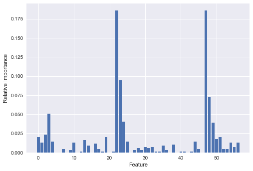
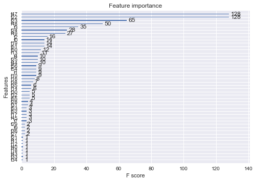
Feature Importance

The basic question to answer is… what is driving these high scores? What features in our dataset are allowing such high predictions?

The answer is … tower kills and inhibitor kills. Not unsurprisingly, the team which destroys the most towers and most inhibitors wins. Given that this is the prime objective of the game, this is not unexpected.

plt.bar(range(len(clf3.feature_importances_)), clf3.feature_importances_)
plt.xlabel("Feature")
plt.ylabel("Relative Importance")
plt.show()

plot_importance(clf3)
plt.show()

png

selection = SelectFromModel(clf3, threshold=0.05, prefit=True)
X_train_sel = selection.transform(X_train)
selection_model = XGBClassifier()
selection_model.fit(select_X_train, y_train)
X_test_sel = selection.transform(X_test)
y_pred = selection_model.predict(X_test_sel)

predictions = [round(value) for value in y_pred]
accuracy = accuracy_score(y_test, predictions)
print("Thresh=%.3f, n=%d, Accuracy: %.2f%%" % (0.05, X_train_sel.shape[1], accuracy*100.0))

Thresh=0.050, n=4, Accuracy: 96.05%

X_new = pd.DataFrame(X.columns)
X_new['importance'] = clf3.feature_importances_
X_new.sort_values(by='importance', ascending=False).head(15)

	0	importance
47	t2_towerKills	0.195015
22	t1_towerKills	0.190616
23	t1_inhibitorKills	0.107038
48	t2_inhibitorKills	0.068915
3	firstInhibitor	0.049853
24	t1_baronKills	0.033724
49	t2_baronKills	0.027859
13	t1_champ3id	0.021994
16	t1_champ4id	0.020528
19	t1_champ5id	0.020528
50	t2_dragonKills	0.017595
2	firstTower	0.017595
51	t2_riftHeraldKills	0.016129
0	gameDuration	0.016129
54	t2_ban3	0.014663

Starting Variables

As stated above, the previous analysis was done on variables which are known at the end of the game. We would expect potentially no predictability given the starting variables. As seen below, this is the case. If we only take variables that are known at the start such as selected champions, summonr spells & team bans, the predictability drops to no better than a coin flip.

This highlights, perhaps, why these RTS games are so popular… no matter what combination of starting variables, the outcome is still highly dependent on individual player skill and how the team comes together. The actual starting selections bare only a marginal impact on the end results.

X_reduced = df.iloc[:, np.r_[10:24, 30:49, 55:59]]
X_reduced = StandardScaler().fit_transform(X_reduced)
X_train, X_test, y_train, y_test = train_test_split(X_reduced, y)

clf = LogisticRegression()
clf.fit(X_train, y_train)

clf3 = XGBClassifier()
clf3.fit(X_train, y_train)

print("Logistic Regr. Score = ", clf.score(X_test, y_test))
print("XGBoost Score = ", clf3.score(X_test, y_test))

Logistic Regr. Score =  0.515135051226
XGBoost Score =  0.519403911829