Horses for Courses: A Systematic Betting Strategy
This dataset has been available for quite some time now, and there are many analyses of it. I’ve gone a similar route… how can we exploit this data for betting purposes. I take an approach from systematic/quantitative portfolio management, and use a factor returns/factor loading approach to determine an “alpha” for each horse in a race and systematically bet across these alphas. This approach looks to systematically exploit inefficiencies in the betting market and bet against other market participants biases. An example of this may be that punters consistently pay a premium to bet on younger horses, perhaps above and beyond the actual age effect in the race.
This approach was heavily inspired by the Macquarie Quant research teams 2017 Melbourne Cup publication which can be found across the web. Unfortunately, I don’t replicate their exceptional returns here (perhaps deliberately) but simply demonstrate how to apply the techniques using Python.
Disclaimer: this is entirely for fun and demonstrative purposes only, I have no experience with horse betting
import pandas as pd
import numpy as np
import matplotlib.pyplot as plt
import seaborn as sns
runners = pd.read_csv(r"D:\Downloads\horses-for-courses (1)\runners.csv")
forms = pd.read_csv(r"D:\Downloads\horses-for-courses (1)\forms.csv")
odds = pd.read_csv(r"D:\Downloads\horses-for-courses (1)\odds.csv")
horses = pd.read_csv(r"D:\Downloads\horses-for-courses (1)\horses.csv")
markets = pd.read_csv(r"D:\Downloads\horses-for-courses (1)\markets.csv")
riders = pd.read_csv(r"D:\Downloads\horses-for-courses (1)\riders.csv")
EDA
runners = runners[['id','position', 'place_paid', 'market_id', 'horse_id', 'trainer_id', 'rider_id', 'form_rating_one', 'handicap_weight', 'barrier', 'last_five_starts']]
forms = forms[['market_id', 'horse_id', 'runner_number','days_since_last_run', 'overall_starts', 'field_strength', 'overall_wins', 'overall_places']]

eda_df = runners.merge(forms, left_on=['market_id', 'horse_id'], right_on=['market_id','horse_id'])
eda_df = eda_df.merge(horses, left_on = ['horse_id'], right_on=['id'])
eda_df = eda_df.merge(riders, left_on = ['rider_id'], right_on=['id'])
odds_mean = odds.groupby(['runner_id']).mean()
odds_mean.reset_index(inplace=True)
eda_df = eda_df.merge(odds_mean, left_on = 'id_x', right_on = 'runner_id')

eda_df.drop(['id_y','id_x', 'odds_one_place_wagered', 'odds_two_place_wagered', 'odds_three_place_wagered', 'odds_two_win_wagered'], axis=1, inplace=True)
eda_df.info()
<class 'pandas.core.frame.DataFrame'>
Int64Index: 80805 entries, 0 to 80804
Data columns (total 40 columns):
position                    61605 non-null float64
place_paid                  80805 non-null int64
market_id                   80805 non-null int64
horse_id                    80805 non-null int64
trainer_id                  80805 non-null float64
rider_id                    80805 non-null object
form_rating_one             80805 non-null float64
handicap_weight             80805 non-null float64
barrier                     80805 non-null int64
last_five_starts            76311 non-null object
runner_number               80805 non-null int64
days_since_last_run         80805 non-null int64
overall_starts              80805 non-null int64
field_strength              79843 non-null float64
overall_wins                80805 non-null int64
overall_places              80805 non-null int64
age                         80805 non-null float64
sex_id                      80805 non-null float64
sire_id                     80805 non-null float64
dam_id                      80805 non-null float64
prize_money                 80805 non-null float64
id                          80805 non-null int64
sex                         80805 non-null object
runner_id                   80805 non-null int64
odds_one_win                80805 non-null float64
odds_one_win_wagered        80805 non-null float64
odds_one_place              80805 non-null float64
odds_one_place_wagered      0 non-null float64
odds_two_win                80805 non-null float64
odds_two_win_wagered        0 non-null float64
odds_two_place              80805 non-null float64
odds_two_place_wagered      0 non-null float64
odds_three_win              80805 non-null float64
odds_three_win_wagered      80805 non-null float64
odds_three_place            80805 non-null float64
odds_three_place_wagered    80805 non-null float64
odds_four_win               80805 non-null float64
odds_four_win_wagered       80805 non-null float64
odds_four_place             80805 non-null float64
odds_four_place_wagered     80805 non-null float64
dtypes: float64(26), int64(11), object(3)
memory usage: 25.3+ MB
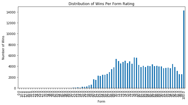
Form Rating
Interestingly, we see that unless the horses form is 100.0, if the horses form is between ~70-99 there is no substantial difference in the number of wins recorded. In fact, there does seem to be a dropoff in the higher form ratings but this could be due to a smaller sample size available. It may also be the fact that form raters are more likely to assign a 100.0 than a 99.0, which leads to the significant uptick in horses being rated 100.0 winning.
form_data = eda_df.groupby(['form_rating_one'])['overall_wins', 'overall_places'].sum()
plt.figure(figsize=(10,5))
form_data['overall_wins'].plot(kind='bar')
plt.ylabel('Number of Wins')
plt.xlabel('Form')
plt.title('Distribution of Wins Per Form Rating')
plt.show()
plt.figure(figsize=(10,5))
form_data['overall_places'].plot(kind='bar')
plt.ylabel('Number of Wins')
plt.xlabel('Form')
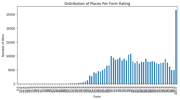
plt.title('Distribution of Places Per Form Rating')
plt.show()
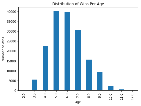
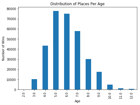
Age
age_data = eda_df.groupby(['age'])['overall_wins', 'overall_places'].sum()
plt.figure(figsize=(7,5))
age_data['overall_wins'].plot(kind='bar')
plt.ylabel('Number of Wins')
plt.xlabel('Age')
plt.title('Distribution of Wins Per Age')
plt.show()

plt.figure(figsize=(7,5))
age_data['overall_places'].plot(kind='bar')
plt.ylabel('Number of Wins')
plt.xlabel('Age')
plt.title('Distribution of Places Per Age')
plt.show()
<matplotlib.figure.Figure at 0x249d062fe48>
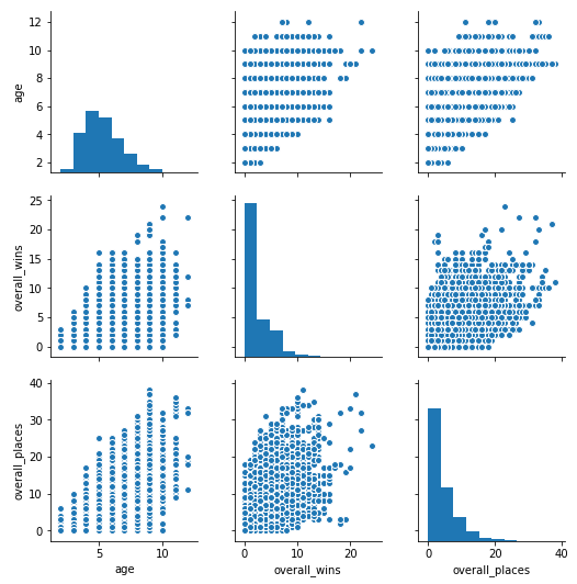
sns.pairplot(eda_df[['age', 'overall_wins', 'overall_places']])
plt.show()
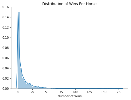
horse_data = pd.DataFrame(eda_df.groupby(['horse_id'])['overall_wins', 'overall_places'].sum())
plt.figure(figsize=(7,5))
sns.distplot(horse_data['overall_wins'].values)
plt.xlabel('Number of Wins')
plt.title('Distribution of Wins Per Horse')
plt.show()
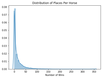
plt.figure(figsize=(7,5))
sns.distplot(horse_data['overall_places'].values)
plt.xlabel('Number of Wins')
plt.title('Distribution of Places Per Horse')
plt.show()
Barriers
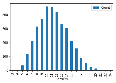
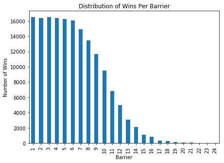
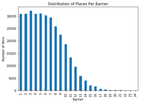
It’s a well known punters strategy to avoid the horses in the outer barriers (i.e. in a 10 barrier race: 8,9, 10). If we look at the distribution of wins/places per barrier, this seems to be reasonably confirmed with barriers 1-6 having a reasonably equal distribution of wins whilst barriers 9-10 drop off substantially. Given that this appears to be a reasonably pervasive anomaly, it should be baked into the odds being offered already, but perhaps there is a systematic bias that punters overestimate the importance of the barrier in the race and this could potentially be exploited.
barrier_data = pd.DataFrame(eda_df.groupby(['barrier'])['overall_wins', 'overall_places'].sum())
barriers_per_race = eda_df.groupby(['market_id'])['barrier'].count()

barrier_counts = pd.DataFrame(list(Counter(barriers_per_race).items()), columns = ['Barriers', 'Count'])
barrier_counts.set_index(['Barriers'], inplace=True)
barrier_counts.plot(kind='bar')
plt.show()
plt.figure(figsize=(7,5))
barrier_data['overall_wins'].plot(kind='bar')
plt.ylabel('Number of Wins')
plt.xlabel('Barrier')
plt.title('Distribution of Wins Per Barrier')
plt.show()

plt.figure(figsize=(7,5))
barrier_data['overall_places'].plot(kind='bar')
plt.ylabel('Number of Wins')
plt.xlabel('Barrier')
plt.title('Distribution of Places Per Barrier')
plt.show()
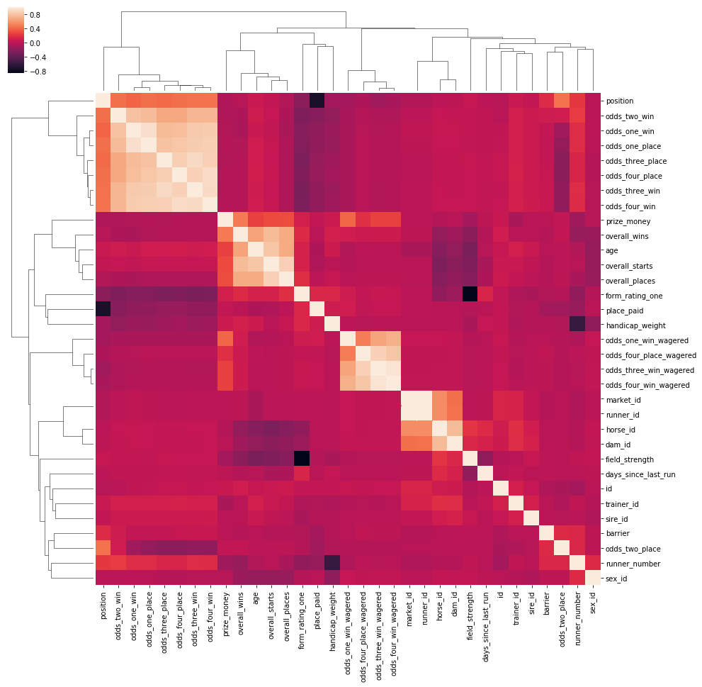
We can see that race position is actually correlated with odds (surprise, surprise).
sns.clustermap(eda_df.corr(), figsize=(15,15))
plt.show()
Betting
We’ll approach developing a betting model similar to what’s known as a factor model in asset management/finance. Our target variable will be the observed return (i.e. if we bet $1 on a horse with odds of 1.5 and the horse wins, our observed return is $0.5) and we’ll use factors such as barrier, age, pre-race odds to try to explain the observed return. By doing this, we may be able to develop a model which can explain the observed return, and then apply this model to new data to attempt to maximise our expected return when betting on a horse race (likely to require us to bet across many horses races… but this is all just for fun!).
forms = forms[['market_id', 'horse_id', 'days_since_last_run']]
runners = runners[['id','position', 'place_paid', 'market_id', 'horse_id','form_rating_one', 'handicap_weight', 'barrier', 'last_five_starts']]

odds_mean = odds.groupby(['runner_id']).mean()
odds_mean.reset_index(inplace=True)
odds_mean = odds_mean[['runner_id', 'odds_one_place', 'odds_two_place', 'odds_three_place', 'odds_four_place']]

combined_df = runners.merge(forms, left_on=['market_id', 'horse_id'], right_on = ['market_id', 'horse_id'])
combined_df = combined_df.merge(odds_mean, left_on = ['id'], right_on = ['runner_id'])
combined_df = combined_df.merge(horses[['id','age']], left_on = 'horse_id', right_on = 'id')
combined_df = combined_df.merge(markets[['id', 'timezone']], left_on='id_x', right_on='id')
combined_df['timezone'] = pd.to_datetime(combined_df['timezone'])
combined_df = combined_df[np.isfinite(combined_df['position'])]

combined_df['odds'] = (combined_df['odds_one_place'] + combined_df['odds_two_place'] + combined_df['odds_three_place'] + combined_df['odds_four_place']) / 4
combined_df.drop(['odds_one_place', 'odds_two_place', 'odds_three_place', 'odds_four_place'], axis=1, inplace=True)
combined_df['return'] = combined_df['place_paid'] * combined_df['odds'] - 1

combined_df['inv_odds'] = 1 / combined_df['odds']
combined_df['inv_odds_sq'] = np.power(combined_df['odds'], 2)

combined_df['last_five_starts'] = combined_df['last_five_starts'].apply(calc_start_score)
to_norm = combined_df[['market_id', 'form_rating_one', 'horse_id','handicap_weight', 'barrier', 'last_five_starts', 'days_since_last_run', 'age', 'inv_odds', 'inv_odds_sq']]
normed_df = to_norm.groupby(['market_id']).apply(lambda x: (x - x.min())/(x.max() - x.min()))
normed_df['market_id'] = combined_df['market_id']
normed_df['timezone'] = combined_df['timezone']
normed_df['horse_id'] = combined_df['horse_id']
normed_df.head()
| market_id | horse_id | handicap_weight | barrier | last_five_starts | days_since_last_run | age | inv_odds | inv_odds_sq | timezone | |
|---|---|---|---|---|---|---|---|---|---|---|
| 4 | 338 | 6 | 0.000000 | 0.153846 | 0.916667 | 0.116667 | 0.250000 | 1.000000 | 0.000000 | 2016-10-02 18:15:00 |
| 6 | 314 | 1 | 1.000000 | 0.250000 | 0.250000 | 0.000000 | 0.571429 | 0.147641 | 0.154099 | 2016-09-27 19:48:00 |
| 9 | 563 | 13 | 0.000000 | 0.090909 | 0.617647 | 0.059633 | 0.600000 | 1.000000 | 0.000000 | 2016-11-25 22:12:00 |
| 22 | 483 | 17 | 0.555556 | 0.727273 | 0.055556 | 0.000000 | 0.000000 | 0.179808 | 0.045073 | 2016-11-21 21:40:00 |
| 27 | 127 | 22 | 0.000000 | 0.909091 | 0.000000 | 0.000000 | 0.000000 | 0.675319 | 0.004061 | 2016-07-30 21:19:00 |
def calc_start_score(value):
    """
    Converts a horse's past 5/20 starts into a numeric score
    i.e. if a horses past races are xf245x, the score should be 15 + 2 + 4 +5 = 26
    f = did not finish, x = scratched.
    """

    arr = list(str(value))
    val = 0
    for i in arr:
        try:
            val += int(i)
        except:
            if i == 'x':
                val += 0
            elif i =='f':
                val += 15
    return val
Factor Loadings
Above we got our data into a nice clean format for running through some regression models. Our approach is fairly simple:
- Split the dataset into a training period (before November 2016) and test period (November 2016 onwards).
- Fit our models to the training dataset. Effectively: $Expected Return = \alpha + \beta_{1}LastFiveStarts + \beta_{2}DaysSinceLastRun + \beta_{3}Handicap + \beta_{4}Barrier + \beta_{5}Form + \beta_{6}\frac{1}{odds} + \beta_{7}\frac{1}{odds}^2 + \epsilon$
- In our test period, calculate the expected return for each horse as $H_{alpha}$ and then bucket our $H_{alpha}$ into quartiles.
- In each race, systematically bet an equal amount across each horse in each quartile
- Track profits over time in each quartile
By doing this, we’ll be able to see if there’s any profit to be made by exploiting our basic model and betting on horses in the top quartile.
from sklearn.linear_model import LinearRegression
from sklearn.model_selection import train_test_split

from xgboost import XGBRegressor
from xgboost import plot_importance
final_df = normed_df.merge(pd.DataFrame(combined_df[['return']]), left_index=True, right_index=True)
final_df.dropna(inplace=True)
train_df = final_df.loc[final_df['timezone'] < '2016-11-01']
test_df = final_df.loc[final_df['timezone'] >= '2016-11-01']
X_train = train_df[['age', 'last_five_starts', 'days_since_last_run', 'handicap_weight', 'barrier', 'form_rating_one', 'inv_odds', 'inv_odds_sq']]
X_test = test_df[['age', 'last_five_starts', 'days_since_last_run', 'handicap_weight', 'barrier', 'form_rating_one', 'inv_odds', 'inv_odds_sq']]

y_train = train_df['return']
y_test = test_df['return']
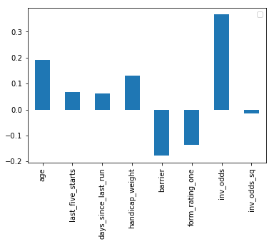
Linear Regression
First we’ll run a linear regression to get an idea of the factor loadings. Effectively this is telling us which factors explained the observed return. We see that inverse odds age and handicap are quite dominant.
model = LinearRegression()
model.fit(X_train.values, y_train.values)
LinearRegression(copy_X=True, fit_intercept=True, n_jobs=1, normalize=False)
pd.DataFrame(model.coef_, X_train.columns).plot(kind='bar')
plt.legend('')
plt.show()
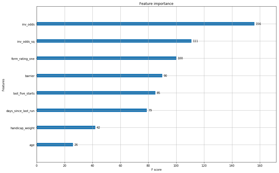
XGBoost
For our actual model, we’ll fit an xgboost random forest regressor.
clf3 = XGBRegressor()
clf3.fit(X_train, y_train)
halphas = pd.DataFrame(clf3.predict(X_test), index=X_test.index, columns=['halpha'])
halphas = halphas.merge(test_df, left_index=True, right_index=True)
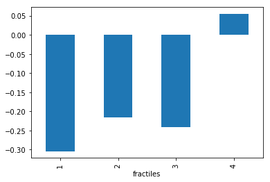
halphas['fractiles'] = halphas.groupby(['market_id'])['halpha'].apply(pd.cut, bins=4, labels=[1,2,3,4])
We notice that are fractiles don’t look particularly good, fractiles 1-3 have a negative mean return, whilst fractile 4 has a slight positive tilt. Ideally we’d liked to have seen fractiles 1/2 with negative returns and fractiles 3/4 with positive returns.
halphas.groupby(['fractiles'])['return'].mean().plot(kind='bar')
plt.show()
ax = plot_importance(clf3)
fig = ax.figure
fig.set_size_inches(15, 10)
plt.show()
Betting Simulation
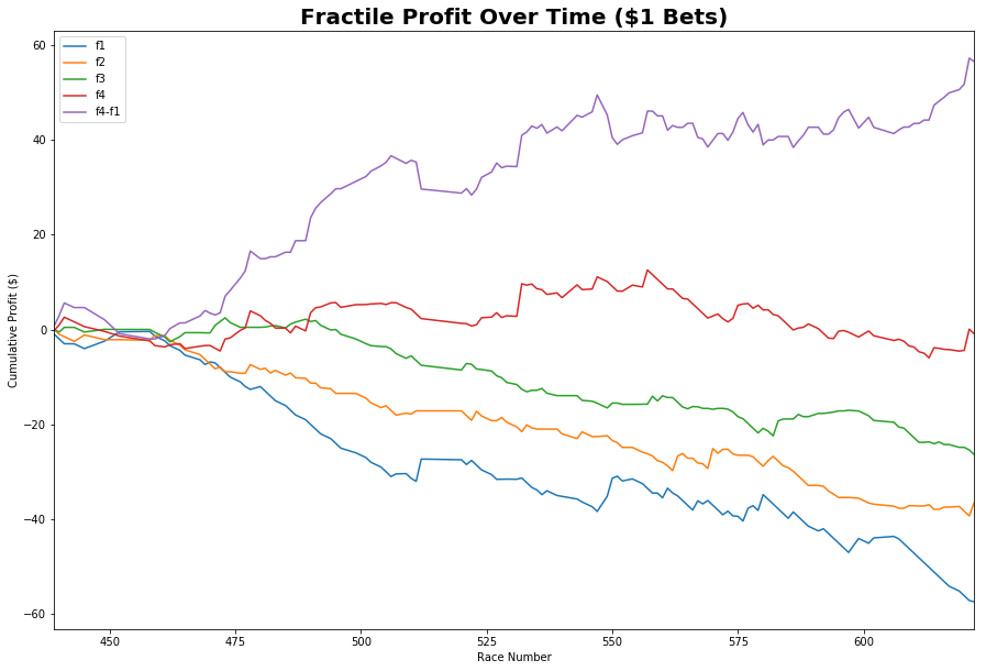
We’ll run our basic betting simulation here, where for each race we distribute a bet equally across the fractiles. We then track our returns over time.
Notice that we do get quite a nice fractile profile spread, where if we could go long our top fractile (fractile 4) and short our bottom fractile (fractile 1) we could make a healthy profit. Unfortunately, I’m not aware of being able to easily bet against a horse.
We thus notice that the top fractile in the long run doesn’t make a huge return. There are numerous reasons for this:
- I’ve only given the model ~135 races to bet on, likely not enough
- My model is fairly naive (deliberately) and I haven’t gone to extra lengths to clean it and deal with outliers etc.
- Potential ways to improve include:
- Bringing in extra factors
- Dealing with missing data better
- Dealing with odds data better: i.e. taking into account time
def sim_bets(df, bet_size):

    results_df = pd.DataFrame()

    for i in np.unique(df['market_id']):
        tmp_df = df.loc[df.market_id == i]

        quint_counts = tmp_df.groupby(['fractiles'])['horse_id'].count()
        bets = pd.DataFrame(bet_size / quint_counts)
        bets.columns = ['bet_amount']

        tmp_df = tmp_df.merge(bets, left_on = 'fractiles', right_index=True)

        tmp_df['bet_return'] = tmp_df['return'] * tmp_df['bet_amount']

        tmp_res = pd.DataFrame(tmp_df.groupby(['fractiles'])['bet_return'].sum())
        tmp_res.fillna(0, inplace=True)
        tmp_res.columns = [i]
        results_df = results_df.append(tmp_res.T)

    return results_df
sim = sim_bets(halphas, 1)
sim_cumu['f4-f1'] = sim_cumu.iloc[:,3] - sim_cumu.iloc[:,0]
sim_cumu = sim.cumsum()
sim_cumu.columns=['f1', 'f2', 'f3', 'f4']
sim_cumu['f4-f1'] = sim_cumu['f4'] - sim_cumu['f1']
sim_cumu.plot(figsize=(15,10))
plt.title('Fractile Profit Over Time ($1 Bets)', size=20, fontweight='bold')
plt.ylabel('Cumulative Profit ($)')
plt.xlabel('Race Number')
plt.show()